安全问题:目前仅仅通过随机 Stream Key 防止未授权推流。
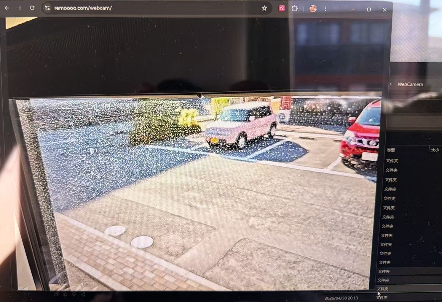
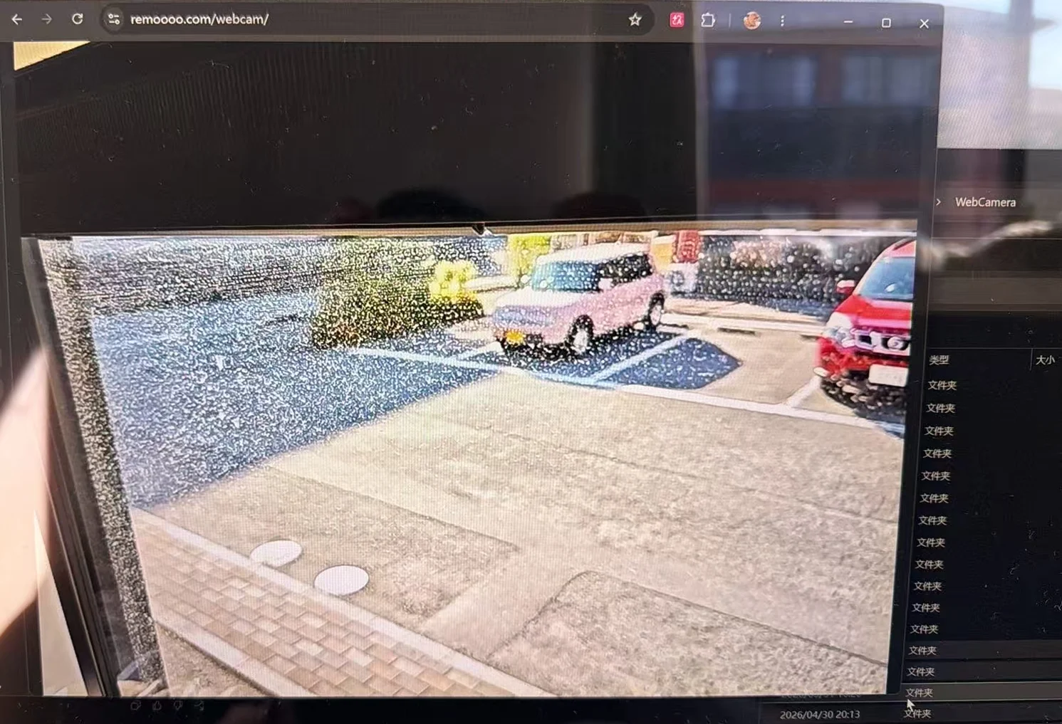
用安卓手机作为摄像头,通过 RTMP 推流到 remoooo.com,并通过 https://remoooo.com/webcam 加密码观看。
Android Phone 通过 RTMP 推流到 Public Server。
Server 端接入 MediaMTX ,转换为 HLS 监听本机地址。
localhost reverse proxy 到 nginx ,用 HTTPS + Basic Auth 最终在 Browser Viewer 查看。
观看入口 rtmp://example.com:1935/
简单的说,服务器端使用 MediaMTX 作为媒体网关。MediaMTX 负责接收手机端 RTMP 推流,并将其转换为浏览器可播放的 HLS 流。
RTMP App:
Protocol: RTMP
Server URL: rtmp://example.com:1935
Stream Key: <stream-key>
Video Codec: H.264
Audio Codec: AAC
Resolution: 1280x720
FPS: 30
Video Bitrate: 2000-3000 kbps
Audio Bitrate: 96-128 kbps
Keyframe Interval: 2s
Bash