Following the previous article

remoooo: Compute Shader Learning Notes (II) Post-processing Effects

L4 particle effects and crowd behavior simulation

This chapter uses Compute Shader to generate particles. Learn how to use DrawProcedural and DrawMeshInstancedIndirect, also known as GPU Instancing.

Summary of knowledge points:

• Compute Shader, Material, C# script and Shader work together
• Graphics.DrawProcedural
• material.SetBuffer()
• xorshift random algorithm
• Swarm Behavior Simulation
• Graphics.DrawMeshInstancedIndirect
• Rotation, translation, and scaling matrices, homogeneous coordinates
• Surface Shader
• ComputeBufferType.Default
• #pragma instancing_options procedural:setup
• unity_InstanceID
• Skinned Mesh Renderer
• Data alignment

1. Introduction and preparation

In addition to being able to process large amounts of data at the same time, Compute Shader also has a key advantage, which is that the Buffer is stored in the GPU. Therefore, the data processed by the Compute Shader can be directly passed to the Shader associated with the Material, that is, the Vertex/Fragment Shader. The key here is that the material can also SetBuffer() like the Compute Shader, accessing data directly from the GPU's Buffer!

Using Compute Shader to create a particle system can fully demonstrate the powerful parallel capabilities of Compute Shader.

During the rendering process, the Vertex Shader reads the position and other attributes of each particle from the Compute Buffer and converts them into vertices on the screen. The Fragment Shader is responsible for generating pixels based on the information of these vertices (such as position and color). Through the Graphics.DrawProcedural method, Unity canDirect RenderingThese vertices processed by the Shader do not require a pre-defined mesh structure and do not rely on the Mesh Renderer, which is particularly effective for rendering a large number of particles.

2. Hello Particle

The steps are also very simple. Define the particle information (position, speed and life cycle) in C#, initialize and pass the data to Buffer, bind Buffer to Compute Shader and Material. In the rendering stage, call Graphics.DrawProceduralNow in OnRenderObject() to achieve efficient particle rendering.

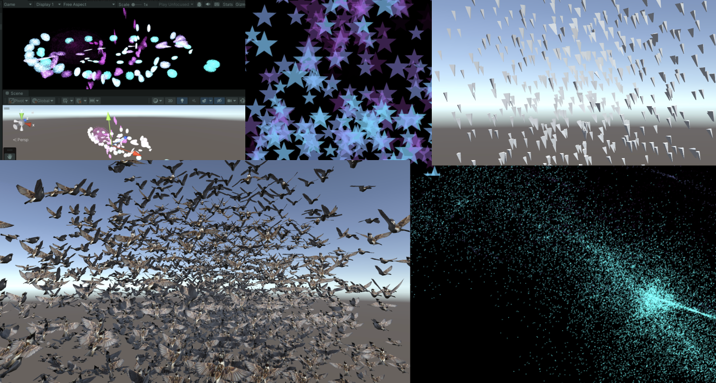
Create a new scene and create an effect: millions of particles follow the mouse and bloom into life, as follows:

Writing this makes me think a lot. The life cycle of a particle is very short, ignited in an instant like a spark, and disappearing like a meteor. Despite thousands of hardships, I am just a speck of dust among billions of dust, ordinary and insignificant. These particles may float randomly in space (Use the "Xorshift" algorithm to calculate the position of particle spawning), may have unique colors, but they can't escape the fate of being programmed. Isn't this a portrayal of my life? I play my role step by step, unable to escape the invisible constraints.

“God is dead! And how can we who have killed him not feel the greatest pain?” – Friedrich Nietzsche

Nietzsche not only announced the disappearance of religious beliefs, but also pointed out the sense of nothingness faced by modern people, that is, without the traditional moral and religious pillars, people feel unprecedented loneliness and lack of direction. Particles are defined and created in the C# script, move and die according to specific rules, which is quite similar to the state of modern people in the universe described by Nietzsche. Although everyone tries to find their own meaning, they are ultimately restricted by broader social and cosmic rules.

Life is full of various inevitable pains, reflecting the inherent emptiness and loneliness of human existence.Particle death logic to be writtenAll of these confirm what Nietzsche said: nothing in life is permanent. The particles in the same buffer will inevitably disappear at some point in the future, which reflects the loneliness of modern people described by Nietzsche. Individuals may feel unprecedented isolation and helplessness, so everyone is a lonely warrior who must learn to face the inner tornado and the indifference of the outside world alone.

But it doesn’t matter, “Summer will come again and again, and those who are meant to meet will meet again.” The particles in this article will also be regenerated after the end, embracing their own Buffer in the best state.

Summer will come around again. People who meet will meet again.

The current version of the code can be copied and run by yourself (all with comments):

• Compute Shader: https://github.com/Remyuu/Unity-Compute-Shader-Learn/blob/L4_First_Particle/Assets/Shaders/ParticleFun.compute
• CPU: https://github.com/Remyuu/Unity-Compute-Shader-Learn/blob/L4_First_Particle/Assets/Scripts/ParticleFun.cs
• Shader: https://github.com/Remyuu/Unity-Compute-Shader-Learn/blob/L4_First_Particle/Assets/Shaders/Particle.shader

Enough of the nonsense, let’s first take a look at how the C# script is written.

As usual, first define the particle buffer (structure), initialize it, and then pass it to the GPU.The key lies in the last three lines that bind the Buffer to the shader operation.There is nothing much to say about the code in the ellipsis below. They are all routine operations, so they are just mentioned with comments.

struct Particle{ public Vector3 position; // Particle positionpublic Vector3 velocity; // Particle velocitypublic float life; // Particle life cycle } ComputeBuffer particleBuffer; // GPU Buffer ... // Init() // Initialize particle array Particle[] particleArray = new Particle[particleCount]; for (int i = 0; i < particleCount; i++){ // Generate random positions and normalize... // Set the initial position and velocity of the particle... // Set the life cycle of the particle particleArray[i].life = Random.value * 5.0f + 1.0f; } // Create and set up the Compute Buffer ... // Find the kernel ID in the Compute Shader ... // Bind the Compute Buffer to the shader shader.SetBuffer(kernelID, "particleBuffer", particleBuffer); material.SetBuffer("particleBuffer", particleBuffer); material.SetInt("_PointSize", pointSize);

The key rendering stage is OnRenderObject(). material.SetPass is used to set the rendering material channel. The DrawProceduralNow method draws geometry without using traditional meshes. MeshTopology.Points specifies the topology type of the rendering as points. The GPU will treat each vertex as a point and will not form lines or faces between vertices. The second parameter 1 means starting drawing from the first vertex. particleCount specifies the number of vertices to render, which is the number of particles, that is, telling the GPU how many points need to be rendered in total.

void OnRenderObject() { material.SetPass(0); Graphics.DrawProceduralNow(MeshTopology.Points, 1, particleCount); }

Get the current mouse position method. OnGUI() This method may be called multiple times per frame. The z value is set to the camera's near clipping plane plus an offset. Here, 14 is added to get a world coordinate that is more suitable for visual depth (you can also adjust it yourself).

void OnGUI() { Vector3 p = new Vector3(); Camera c = Camera.main; Event e = Event.current; Vector2 mousePos = new Vector2(); // Get the mouse position from Event. // Note that the y position from Event is inverted. mousePos.x = e.mousePosition.x; mousePos.y = c.pixelHeight - e.mousePosition.y; p = c.ScreenToWorldPoint(new Vector3(mousePos.x, mousePos.y, c.nearClipPlane + 14)); cursorPos.x = px; cursorPos.y = py; }

ComputeBuffer particleBuffer has been passed to Compute Shader and Shader above.

Let's first look at the data structure of the Compute Shader. Nothing special.

// Define particle data structure struct Particle { float3 position; // particle position float3 velocity; // particle velocity float life; // particle remaining life time }; // Structured buffer used to store and update particle data, which can be read and written from GPU RWStructuredBuffer particleBuffer; // Variables set from the CPU float deltaTime; // Time difference from the previous frame to the current frame float2 mousePosition; // Current mouse position

Here I will briefly talk about a particularly useful random number sequence generation method, the xorshift algorithm. It will be used to randomly control the movement direction of particles as shown above. The particles will move randomly in three-dimensional directions.

• For more information, please refer to: https://en.wikipedia.org/wiki/Xorshift
• Original paper link: https://www.jstatsoft.org/article/view/v008i14

This algorithm was proposed by George Marsaglia in 2003. Its advantages are that it is extremely fast and very space-efficient. Even the simplest Xorshift implementation has a very long pseudo-random number cycle.

The basic operations are shift and XOR. Hence the name of the algorithm. Its core is to maintain a non-zero state variable and generate random numbers by performing a series of shift and XOR operations on this state variable.

// State variable for random number generation uint rng_state; uint rand_xorshift() { // Xorshift algorithm from George Marsaglia's paper rng_state ^= (rng_state << 13); // Shift the state variable left by 13 bits, then XOR it with the original state rng_state ^= (rng_state >> 17); // Shift the updated state variable right by 17 bits, and XOR it again rng_state ^= (rng_state << 5); // Finally, shift the state variable left by 5 bits, and XOR it one last time return rng_state; // Return the updated state variable as the generated random number }

Basic Xorshift The core of the algorithm has been explained above, but different shift combinations can create multiple variants. The original paper also mentions the Xorshift128 variant. Using a 128-bit state variable, the state is updated by four different shifts and XOR operations. The code is as follows:

// c language Ver uint32_t xorshift128(void) { static uint32_t x = 123456789; static uint32_t y = 362436069; static uint32_t z = 521288629; static uint32_t w = 88675123; uint32_t t = x ^ (x << 11); x = y; y = z; z = w; w = w ^ (w >> 19) ^ (t ^ (t >> 8)); return w; }

This can produce longer periods and better statistical performance. The period of this variant is close, which is very impressive.

In general, this algorithm is completely sufficient for game development, but it is not suitable for use in fields such as cryptography.

When using this algorithm in Compute Shader, you need to pay attention to the range of random numbers generated by the Xorshift algorithm when it is the range of uint32, and you need to do another mapping ([0, 2^32-1] is mapped to [0, 1]):

float tmp = (1.0 / 4294967296.0); // conversion factor rand_xorshift()) * tmp

The direction of particle movement is signed, so we just need to subtract 0.5 from it. Random movement in three directions:

float f0 = float(rand_xorshift()) * tmp - 0.5; float f1 = float(rand_xorshift()) * tmp - 0.5; float f2 = float(rand_xorshift()) * tmp - 0.5; float3 normalF3 = normalize(float3(f0, f1, f2)) * 0.8f; // Scaled the direction of movement

Each Kernel needs to complete the following:

• First get the particle information of the previous frame in the Buffer
• Maintain particle buffer (calculate particle velocity, update position and health value), write back to buffer
• If the health value is less than 0, regenerate a particle

Generate particles. Use the random number obtained by Xorshift just now to define the particle's health value and reset its speed.

// Set the new position and life of the particle particleBuffer[id].position = float3(normalF3.x + mousePosition.x, normalF3.y + mousePosition.y, normalF3.z + 3.0); particleBuffer[id].life = 4; // Reset life particleBuffer[id].velocity = float3(0,0,0); // Reset velocity

Finally, the basic data structure of Shader:

struct Particle{ float3 position; float3 velocity; float life; }; struct v2f{ float4 position : SV_POSITION; float4 color : COLOR; float life : LIFE; float size: PSIZE; }; // particles' data StructuredBuffer particleBuffer;

Then the vertex shader calculates the vertex color of the particle, the Clip position of the vertex, and transmits the information of a vertex size.

v2f vert(uint vertex_id : SV_VertexID, uint instance_id : SV_InstanceID){ v2f o = (v2f)0; // Color float life = particleBuffer[instance_id].life; float lerpVal = life * 0.25f; o.color = fixed4(1.0 f - lerpVal+0.1, lerpVal+0.1, 1.0f, lerpVal); // Position o.position = UnityObjectToClipPos(float4(particleBuffer[instance_id].position, 1.0f)); o.size = _PointSize; return o; }

The fragment shader calculates the interpolated color.

float4 frag(v2f i) : COLOR{ return i.color; }

At this point, you can get the above effect.

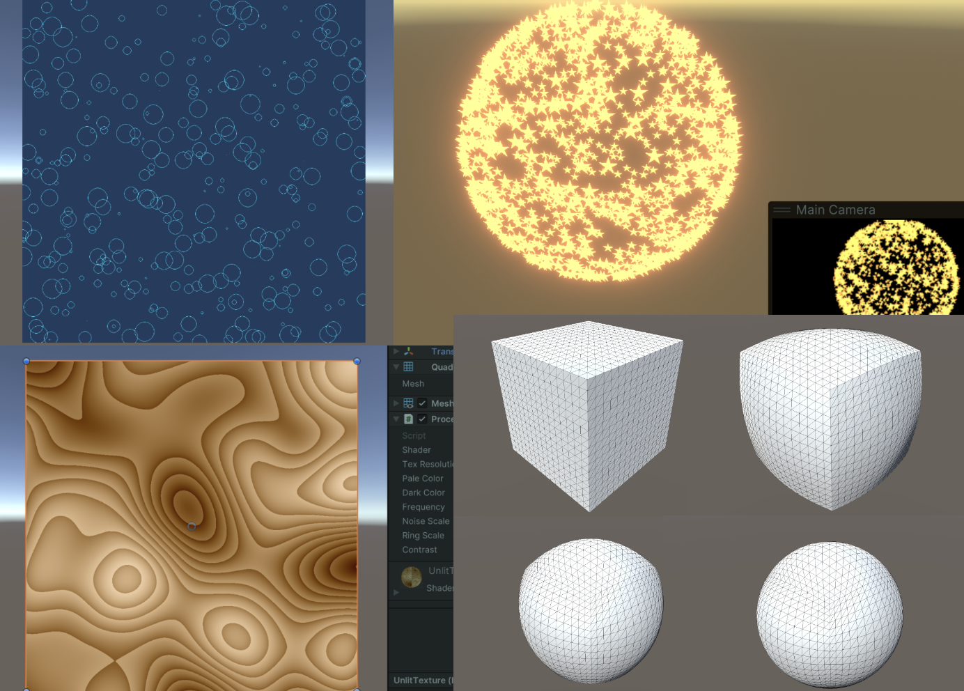
3. Quad particles

In the previous section, each particle only had one point, which was not interesting. Now let's turn a point into a Quad. In Unity, there is no Quad, only a fake Quad composed of two triangles.

Let's start working on it, based on the code above. Define the vertices in C#, the size of a Quad.

// struct struct Vertex { public Vector3 position; public Vector2 uv; public float life; } const int SIZE_VERTEX = 6 * sizeof(float); public float quadSize = 0.1f; // Quad size

On a per-particle basis, set the UV coordinates of the six vertices for use in the vertex shader, and draw them in the order specified by Unity.

index = i*6; //Triangle 1 - bottom-left, top-left, top-right vertexArray[index].uv.Set(0,0); vertexArray[index+1].uv.Set(0,1 ); vertexArray[index+2].uv.Set(1,1); //Triangle 2 - bottom-left, top-right, bottom-right vertexArray[index+3].uv.Set(0,0); vertexArray[index+4].uv.Set(1,1); vertexArray[index+5].uv.Set(1,0);

Finally, it is passed to Buffer. The halfSize here is used to pass to Compute Shader to calculate the positions of each vertex of Quad.

vertexBuffer = new ComputeBuffer(numVertices, SIZE_VERTEX); vertexBuffer.SetData(vertexArray); shader.SetBuffer(kernelID, "vertexBuffer", vertexBuffer); shader.SetFloat("halfSize", quadSize*0.5f); material.SetBuffer("vertexBuffer ", vertexBuffer);

During the rendering phase, the points are changed into triangles with six points.

void OnRenderObject() { material.SetPass(0); Graphics.DrawProceduralNow(MeshTopology.Triangles, 6, numParticles); }

Change the settings in the Shader to receive vertex data and a texture for display. Alpha culling is required.

_MainTex("Texture", 2D) = "white" {} ... Tags{ "Queue"="Transparent" "RenderType"="Transparent" "IgnoreProjector"="True" } LOD 200 Blend SrcAlpha OneMinusSrcAlpha ZWrite Off .. . struct Vertex{ float3 position; float2 uv; float life; }; StructuredBuffer vertexBuffer; sampler2D _MainTex; v2f vert(uint vertex_id : SV_VertexID, uint instance_id : SV_InstanceID) { v2f o = (v2f)0; int index = instance_id*6 + vertex_id; float lerpVal = vertexBuffer[index].life * 0.25f; o .color = fixed4(1.0f - lerpVal+0.1, lerpVal+0.1, 1.0f, lerpVal); o.position = UnityWorldToClipPos(float4(vertexBuffer[index].position, 1.0f)); o.uv = vertexBuffer[index].uv; return o; } float4 frag(v2f i) : COLOR { fixed4 color = tex2D( _MainTex, i.uv ) * i.color; return color; }

In the Compute Shader, add receiving vertex data and halfSize.

struct Vertex { float3 position; float2 uv; float life; }; RWStructuredBuffer vertexBuffer; float halfSize;

Calculate the positions of the six vertices of each Quad.

//Set the vertex buffer // int index = id.x * 6; //Triangle 1 - bottom-left, top-left, top-right vertexBuffer[index].position.x = p.position.x-halfSize; vertexBuffer[index].position.y = p.position.y-halfSize; vertexBuffer[index].position.z = p.position.z; vertexBuffer[index].life = p.life; vertexBuffer[index+1].position.x = p.position.x-halfSize; vertexBuffer[index+1].position.y = p.position.y+halfSize; vertexBuffer[index+1].position.z = p .position.z; vertexBuffer[index+1].life = p.life; vertexBuffer[index+2].position.x = p.position.x+halfSize; vertexBuffer[index+2].position.y = p.position.y+halfSize; vertexBuffer[index+2].position.z = p.position.z; vertexBuffer[index+2].life = p.life; //Triangle 2 - bottom-left, top-right, bottom-right // // vertexBuffer[index+3].position.x = p.position.x-halfSize; vertexBuffer[index+3].position.y = p.position.y-halfSize; vertexBuffer[index+3].position.z = p.position.z; vertexBuffer[index+3].life = p.life; vertexBuffer[index+4].position.x = p.position.x+halfSize; vertexBuffer[index+4].position.y = p.position.y+halfSize ; vertexBuffer[index+4].position.z = p.position.z; vertexBuffer[index+4].life = p.life; vertexBuffer[index+5].position.x = p.position.x+halfSize; vertexBuffer[index+5].position.y = p.position.y-halfSize; vertexBuffer[index+5].position.z = p.position.z; vertexBuffer[index+5].life = p.life;

Mission accomplished.

Current version code:

• Compute Shader: https://github.com/Remyuu/Unity-Compute-Shader-Learn/blob/L4_Quad/Assets/Shaders/QuadParticles.compute
• CPU: https://github.com/Remyuu/Unity-Compute-Shader-Learn/blob/L4_Quad/Assets/Scripts/QuadParticles.cs
• Shader: https://github.com/Remyuu/Unity-Compute-Shader-Learn/blob/L4_Quad/Assets/Shaders/QuadParticle.shader

In the next section, we will upgrade the Mesh to a prefab and try to simulate the flocking behavior of birds in flight.

4. Flocking simulation

Flocking is an algorithm that simulates the collective movement of animals such as flocks of birds and schools of fish in nature. The core is based on three basic behavioral rules, proposed by Craig Reynolds in Sig 87, and is often referred to as the "Boids" algorithm:

• Separation Particles cannot be too close to each other, and there must be a sense of boundary. Specifically, the particles with a certain radius around them are calculated and then a direction is calculated to avoid collision.
• Alignment The speed of an individual tends to the average speed of the group, and there should be a sense of belonging. Specifically, the average speed of particles within the visual range is calculated (the speed size direction). This visual range is determined by the actual biological characteristics of the bird, which will be mentioned in the next section.
• Cohesion The position of the individual particles tends to the average position (the center of the group) to feel safe. Specifically, each particle finds the geometric center of its neighbors and calculates a moving vector (the final result is the averageLocation).

Think about it, which of the above three rules is the most difficult to implement?

Answer: Separation. As we all know, calculating collisions between objects is very difficult to achieve. Because each individual needs to compare distances with all other individuals, this will cause the time complexity of the algorithm to be close to O(n^2), where n is the number of particles. For example, if there are 1,000 particles, then nearly 500,000 distance calculations may be required in each iteration. In the original paper, the author took 95 seconds to render one frame (80 birds) in the original unoptimized algorithm (time complexity O(N^2)), and it took nearly 9 hours to render a 300-frame animation.

Generally speaking, using a quadtree or spatial hashing method can optimize the calculation. You can also maintain a neighbor list to store the individuals around each individual at a certain distance. Of course, you can also use Compute Shader to perform hard calculations.

Without further ado, let’s get started.

First download the prepared project files (if not prepared in advance):

• Bird's Prefab: https://github.com/Remyuu/Unity-Compute-Shader-Learn/blob/main/Assets/Prefabs/Boid.prefab
• Script: https://github.com/Remyuu/Unity-Compute-Shader-Learn/blob/main/Assets/Scripts/SimpleFlocking.cs
• Compute Shader: https://github.com/Remyuu/Unity-Compute-Shader-Learn/blob/main/Assets/Shaders/SimpleFlocking.compute

Then add it to an empty GO.

Start the project and you'll see a bunch of birds.

Below are some parameters for group behavior simulation.

// Define the parameters for the crowd behavior simulation. public float rotationSpeed = 1f; // Rotation speed. public float boidSpeed = 1f; // Boid speed. public float neighbourDistance = 1f; // Neighboring distance. public float boidSpeedVariation = 1f; // Speed variation. public GameObject boidPrefab; // Prefab of Boid object. public int boidsCount; // Number of Boids. public float spawnRadius; // Radius of Boid spawn. public Transform target; // The moving target of the crowd.

Except for the Boid prefab boidPrefab and the spawn radius spawnRadius, everything else needs to be passed to the GPU.

For the sake of convenience, let’s make a foolish mistake in this section. We will only calculate the bird’s position and direction on the GPU, and then pass it back to the CPU for the following processing:

... boidsBuffer.GetData(boidsArray); // Update the position and direction of each bird for (int i = 0; i < boidsArray.Length; i++){ boids[i].transform.localPosition = boidsArray[i].position; if (!boidsArray[i].direction.Equals(Vector3.zero)){ boids[i].transform.rotation = Quaternion.LookRotation(boidsArray[i].direction); } }

The Quaternion.LookRotation() method is used to create a rotation so that an object faces a specified direction.

Calculate the position of each bird in the Compute Shader.

#pragma kernel CSMain #define GROUP_SIZE 256 struct Boid{ float3 position; float3 direction; }; RWStructuredBuffer boidsBuffer; float time; float deltaTime; float rotationSpeed; float boidSpeed; float boidSpeedVariation; float3 flockPosition; float neighborDistance; int boidsCount;

[numthreads(GROUP_SIZE,1,1)]

void CSMain (uint3 id : SV_DispatchThreadID) { … // Continue below }

First write the logic of alignment and aggregation, and finally output the actual position and direction to the Buffer.

Boid boid = boidsBuffer[id.x]; float3 separation = 0; // Separation float3 alignment = 0; // Alignment - direction float3 cohesion = flockPosition; // Aggregation - position uint nearbyCount = 1; // Count itself as a surrounding individual. for (int i=0; i

This is the result of having no sense of boundaries (separation terms), all individuals appear to have a fairly close relationship and overlap.

Add the following code.

if(distance(boid.position, temp.position)< neighborDistance) { float3 offset = boid.position - temp.position; float dist = length(offset); if(dist < neighborDistance) { dist = max(dist, 0.000001) ; separation += offset * (1.0/dist - 1.0/neighbourDistance); } ...

1.0/dist When the Boids are closer together, this value is larger, indicating that the separation force should be greater. 1.0/neighbourDistance is a constant based on the defined neighbor distance. The difference between the two represents how much the actual separation force responds to the distance. If the distance between the two Boids is exactly neighborDistance, this value is zero (no separation force). If the distance between the two Boids is less than neighborDistance, this value is positive, and the smaller the distance, the larger the value.

Current code: https://github.com/Remyuu/Unity-Compute-Shader-Learn/blob/L4_Flocking/Assets/Shaders/SimpleFlocking.compute

The next section will use Instanced Mesh to improve performance.

5. GPU Instancing Optimization

First, let's review the content of this chapter. In both the "Hello Particle" and "Quad Particle" examples, we used the Instanced technology (Graphics.DrawProceduralNow()) to pass the particle position calculated by the Compute Shader directly to the VertexFrag shader.

DrawMeshInstancedIndirect used in this section is used to draw a large number of geometric instances. The instances are similar, but the positions, rotations or other parameters are slightly different. Compared with DrawProceduralNow, which regenerates the geometry and renders it every frame, DrawMeshInstancedIndirect only needs to set the instance information once, and then the GPU can render all instances at once based on this information. Use this function to render grass and groups of animals.

This function has many parameters, only some of which are used.

Graphics.DrawMeshInstancedIndirect(boidMesh, 0, boidMaterial, bounds, argsBuffer);

1. boidMesh: Throw the bird Mesh in.
2. subMeshIndex: The submesh index to draw. Usually 0 if the mesh has only one submesh.
3. boidMaterial: The material applied to the instanced object.
4. Bounds: The bounding box specifies the drawing range. The instantiated object will only be rendered in the area within this bounding box. Used to optimize performance.
5. argsBuffer: ComputeBuffer of parameters, including the number of indices of each instance's geometry and the number of instances.

What is this argsBuffer? This parameter is used to tell Unity which mesh we want to render and how many meshes we want to render! We can use a special Buffer as a parameter.

When initializing the shader, a special Buffer is created, which is labeled ComputeBufferType.IndirectArguments. This type of buffer is specifically used to pass to the GPU so that indirect drawing commands can be executed on the GPU. The first parameter of new ComputeBuffer here is 1, which represents an args array (an array has 5 uints). Don't get it wrong.

ComputeBuffer argsBuffer; ... argsBuffer = new ComputeBuffer(1, 5 * sizeof(uint), ComputeBufferType.IndirectArguments); if (boidMesh != null) { args[0] = (uint)boidMesh.GetIndexCount(0); args[ 1] = (uint)numOfBoids; } argsBuffer.SetData(args); ... Graphics.DrawMeshInstancedIndirect(boidMesh, 0, boidMaterial, bounds, argsBuffer);

Based on the previous chapter, an offset is added to the individual data structure, which is used for the direction offset in the Compute Shader. In addition, the direction of the initial state is interpolated using Slerp, 70% keeps the original direction, and 30% is random. The result of Slerp interpolation is a quaternion, which needs to be converted to Euler angles using the quaternion method and then passed into the constructor.

public float noise_offset; ... Quaternion rot = Quaternion.Slerp(transform.rotation, Random.rotation, 0.3f); boidsArray[i] = new Boid(pos, rot.eulerAngles, offset);

After passing this new attribute noise_offset to the Compute Shader, a noise value in the range [-1, 1] is calculated and applied to the bird's speed.

float noise = clamp(noise1(time / 100.0 + boid.noise_offset), -1, 1) * 2.0 - 1.0; float velocity = boidSpeed * (1.0 + noise * boidSpeedVariation);

Then we optimized the algorithm a bit. Compute Shader is basically the same.

if (distance(boid_pos, boidsBuffer[i].position) < neighborDistance) { float3 tempBoid_position = boidsBuffer[i].position; float3 offset = boid.position - tempBoid_position; float dist = length(offset); if (dist

The biggest difference is in the shader. This section uses a surface shader instead of a fragment. This is actually a packaged vertex and fragment shader. Unity has already done a lot of tedious work such as lighting and shadows. You can still specify a vertice.

When writing shaders to make materials, you need to do special processing for instanced objects. Because the positions, rotations and other properties of ordinary rendering objects are static in Unity. For the instantiated objects to be built, their positions, rotations and other parameters are constantly changing. Therefore, a special mechanism is needed in the rendering pipeline to dynamically set the position and parameters of each instantiated object. The current method is based on the instantiation technology of the program, which can render all instantiated objects at once without drawing them one by one. That is, one-time batch rendering.

The shader uses the instanced technique. The instantiation phase is executed before vert. This way each instantiated object has its own rotation, translation, and scaling matrices.

Now we need to create a rotation matrix for each instantiated object. From the Buffer, we get the basic information of the bird calculated by the Compute Shader (in the previous section, the data was sent back to the CPU, and here it is directly sent to the Shader for instantiation):

In Shader, the data structure and related operations passed by Buffer are wrapped with the following macros.

// .shader #ifdef UNITY_PROCEDURAL_INSTANCING_ENABLED struct Boid { float3 position; float3 direction; float noise_offset; }; StructuredBuffer boidsBuffer; #endif

Since I only specified the number of birds to be instantiated (the number of birds, which is also the size of the Buffer) in args[1] of DrawMeshInstancedIndirect of C#, I can directly access the Buffer using the unity_InstanceID index.

#pragma instancing_options procedural:setup void setup() { #ifdef UNITY_PROCEDURAL_INSTANCING_ENABLED _BoidPosition = boidsBuffer[unity_InstanceID].position; _Matrix = create_matrix(boidsBuffer[unity_InstanceID].position, boidsBuffer[unity_InstanceID].direction, float3(0.0, 1.0, 0.0)); #endif }

The calculation of the space transformation matrix here involvesHomogeneous Coordinates, you can review the GAMES101 course. The point is (x,y,z,1) and the coordinates are (x,y,z,0).

If you use affine transformations, the code is as follows:

void setup() { #ifdef UNITY_PROCEDURAL_INSTANCING_ENABLED _BoidPosition = boidsBuffer[unity_InstanceID].position; _LookAtMatrix = look_at_matrix(boidsBuffer[unity_InstanceID].direction, float3(0.0, 1.0, 0.0)); #endif } void vert(inout appdata_full v, out Input data) { UNITY_INITIALIZE_OUTPUT(Input, data); #ifdef UNITY_PROCEDURAL_INSTANCING_ENABLED v.vertex = mul(_LookAtMatrix, v.vertex); v.vertex.xyz += _BoidPosition; #endif }

Not elegant enough, we can just use homogeneous coordinates. One matrix handles rotation, translation and scaling!

void setup() { #ifdef UNITY_PROCEDURAL_INSTANCING_ENABLED _BoidPosition = boidsBuffer[unity_InstanceID].position; _Matrix = create_matrix(boidsBuffer[unity_InstanceID].position, boidsBuffer[unity_InstanceID].direction, float3(0.0, 1.0, 0.0)); #endif } void vert(inout appdata_full v, out Input data) { UNITY_INITIALIZE_OUTPUT(Input, data); #ifdef UNITY_PROCEDURAL_INSTANCING_ENABLED v.vertex = mul(_Matrix, v.vertex); #endif }

Now, we are done! The current frame rate is nearly doubled compared to the previous section.

Current version code:

• Compute Shader: https://github.com/Remyuu/Unity-Compute-Shader-Learn/blob/L4_Instanced/Assets/Shaders/InstancedFlocking.compute
• CPU: https://github.com/Remyuu/Unity-Compute-Shader-Learn/blob/L4_Instanced/Assets/Scripts/InstancedFlocking.cs
• Shader: https://github.com/Remyuu/Unity-Compute-Shader-Learn/blob/L4_Instanced/Assets/Shaders/InstancedFlocking.shader

6. Apply skin animation

What we need to do in this section is to use the Animator component to grab the Mesh of each keyframe into the Buffer before instantiating the object. By selecting different indexes, we can get Mesh of different poses. The specific skeletal animation production is beyond the scope of this article.

You just need to modify the code based on the previous chapter and add the Animator logic. I have written comments below, you can take a look.

And the individual data structure is updated:

struct Boid{ float3 position; float3 direction; float noise_offset; float speed; // not useful for now float frame; // indicates the current frame index in the animation float3 padding; // ensure data alignment };

Let's talk about alignment in detail. In a data structure, the size of the data should preferably be an integer multiple of 16 bytes.

• float3 position; (12 bytes)
• float3 direction; (12 bytes)
• float noise_offset; (4 bytes)
• float speed; (4 bytes)
• float frame; (4 bytes)
• float3 padding; (12 bytes)

Without padding, the size is 36 bytes, which is not a common alignment size. With padding, the alignment is 48 bytes, perfect!

private SkinnedMeshRenderer boidSMR; // Used to reference the SkinnedMeshRenderer component that contains the skinned mesh. private Animator animator; public AnimationClip animationClip; // Specific animation clips, usually used to calculate animation-related parameters. private int numOfFrames; // The number of frames in the animation, used to determine how many frames of data to store in the GPU buffer. public float boidFrameSpeed = 10f; // Controls the speed at which the animation plays. MaterialPropertyBlock props; // Pass parameters to the shader without creating a new material instance. This means that the material properties of the instance (such as color, lighting coefficient, etc.) can be changed without affecting other objects using the same material. Mesh boidMesh; // Stores the mesh data baked from the SkinnedMeshRenderer. ... void Start(){ // First initialize the Boid data here, then call GenerateSkinnedAnimationForGPUBuffer to prepare the animation data, and finally call InitShader to set the Shader parameters required for rendering. ... // This property block is used only for avoiding an instancing bug. props = new MaterialPropertyBlock(); props.SetFloat("_UniqueID", Random.value); ... InitBoids(); GenerateSkinnedAnimationForGPUBuffer(); InitShader(); } void InitShader(){ // This method configures the Shader and material properties to ensure that the animation playback can be displayed correctly according to the different stages of the instance. Enabling or disabling frameInterpolation determines whether to interpolate between animation frames for smoother animation effects. ... if (boidMesh)//Set by the GenerateSkinnedAnimationForGPUBuffer ... shader.SetFloat("boidFrameSpeed", boidFrameSpeed); shader.SetInt("numOfFrames", numOfFrames); boidMaterial.SetInt("numOfFrames", numOfFrames); if (frameInterpolation && !boidMaterial.IsKeywordEnabled("FRAME_INTERPOLATION")) boidMaterial.EnableKeyword("FRAME_INTERPOLATION"); if (!frameInterpolation && boidMaterial.IsKeywordEnabled("FRAME_INTERPOLATION")) boidMaterial.DisableKeyword("FRAME_INTERPOLATION"); } void Update(){ ... // The last two parameters: // 1. 0: Offset into the parameter buffer, used to specify where to start reading parameters. // 2. props: The MaterialPropertyBlock created earlier, containing properties shared by all instances. Graphics.DrawMeshInstancedIndirect( boidMesh, 0, boidMaterial, bounds, argsBuffer, 0, props); } void OnDestroy(){ ... if (vertexAnimationBuffer != null) vertexAnimationBuffer.Release(); } private void GenerateSkinnedAnimationForGPUBuffer() { ... // Continued }

In order to provide the Shader with Mesh with different postures at different times, the mesh vertex data of each frame is extracted from the Animator and SkinnedMeshRenderer in the GenerateSkinnedAnimationForGPUBuffer() function, and then the data is stored in the GPU's ComputeBuffer for use in instanced rendering.

GetCurrentAnimatorStateInfo to obtain the state information of the current animation layer for subsequent precise control of animation playback.

numOfFrames is determined using the power of two that is closest to the product of the animation length and the frame rate, which can optimize GPU memory access.

Then create a ComputeBuffer to store all vertex data for all frames. vertexAnimationBuffer

In the for loop, bake all animation frames. Specifically, play and update immediately at each sampleTime point, then bake the mesh of the current animation frame into bakedMesh. And extract the newly baked Mesh vertices, update them into the array vertexAnimationData, and finally upload them to the GPU to end.

// ...continued from above boidSMR = boidObject.GetComponentInChildren (); boidMesh = boidSMR.sharedMesh; animator = boidObject.GetComponentInChildren (); int iLayer = 0; AnimatorStateInfo aniStateInfo = animator.GetCurrentAnimatorStateInfo(iLayer); Mesh bakedMesh = new Mesh(); float sampleTime = 0; float perFrameTime = 0; numOfFrames = Mathf.ClosestPowerOfTwo((int)(animationClip.frameRate * animationClip.length)); perFrameTime = animationClip.length / numOfFrames; var vertexCount = boidSMR.sharedMesh.vertexCount; vertexAnimationBuffer = new ComputeBuffer(vertexCount * numOfFrames, 16); Vector4[] vertexAnimationData = new Vector4[vertexCount * numOfFrames]; for (int i = 0; i < numOfFrames; i++) { animator.Play(aniStateInfo.shortNameHash, iLayer, sampleTime); animator.Update(0f); boidSMR.BakeMesh(bakedMesh); for(int j = 0; j < vertexCount; j++) { Vector4 vertex = bakedMesh.vertices[j]; vertex.w = 1; vertexAnimationData[(j * numOfFrames) + i] = vertex; } sampleTime += perFrameTime; } vertexAnimationBuffer.SetData(vertexAnimationData); boidMaterial.SetBuffer("vertexAnimation", vertexAnimationBuffer); boidObject.SetActive(false);

In the Compute Shader, maintain each frame variable stored in an individual data structure.

boid.frame = boid.frame + velocity * deltaTime * boidFrameSpeed; if (boid.frame >= numOfFrames) boid.frame -= numOfFrames;

Lerp different frames of animation in Shader. The left side is without frame interpolation, and the right side is after interpolation. The effect is very significant.

A good title can get more recommendations and followers

void vert(inout appdata_custom v) { #ifdef UNITY_PROCEDURAL_INSTANCING_ENABLED #ifdef FRAME_INTERPOLATION v.vertex = lerp(vertexAnimation[v.id * numOfFrames + _CurrentFrame], vertexAnimation[v.id * numOfFrames + _NextFrame], _FrameInterpolation); #else v.vertex = vertexAnimation[v.id * numOfFrames + _CurrentFrame]; #endif v.vertex = mul(_Matrix, v.vertex); #endif } void setup() { #ifdef UNITY_PROCEDURAL_INSTANCING_ENABLED _Matrix = create_matrix(boidsBuffer[unity_InstanceID].position, boidsBuffer[unity_InstanceID].direction, float3(0.0, 1.0, 0.0)); _CurrentFrame = boidsBuffer[unity_InstanceID].frame; #ifdef FRAME_INTERPOLATION _NextFrame = _CurrentFrame + 1; if (_NextFrame >= numOfFrames) _NextFrame = 0; _FrameInterpolation = frac(boidsBuffer[unity_InstanceID].frame); #endif #endif }

It was not easy, but it is finally complete.

Complete project link: https://github.com/Remyuu/Unity-Compute-Shader-Learn/tree/L4_Skinned/Assets/Scripts

8. Summary/Quiz

When rendering points which gives the best answer?

What are the three key steps in flocking?

When creating an arguments buffer for DrawMeshInstancedIndirect, how many uints are required?

We created the wing flapping by using a skinned mesh shader. True or False.

In a shader used by DrawMeshInstancedIndirect, which variable name gives the correct index for the instance?

References

1. https://en.wikipedia.org/wiki/Boids
2. Flocks, Herds, and Schools: A Distributed Behavioral Model

Preface

Get a preliminary understanding of Compute Shader and implement some simple effects. All the codes are in:

https://github.com/Remyuu/Unity-Compute-Shader-Learngithub.com/Remyuu/Unity-Compute-Shader-Learn

The main branch is the initial code. You can download the complete project and follow me. PS: I have opened a separate branch for each version of the code.

This article learns how to use Compute Shader to make:

• Post-processing effects
• Particle System

The previous article did not mention the GPU architecture because I felt that it would be difficult to understand if I explained a bunch of terms right at the beginning. With the experience of actually writing Compute Shader, you can connect the abstract concepts with the actual code.

CUDA on GPUExecution ProgramIt can be explained by a three-tier architecture:

• Grid – corresponds to a Kernel
• |-Block – A Grid has multiple Blocks, executing the same program
• | |-Thread – The most basic computing unit on the GPU

Thread is the most basic unit of GPU, and there will naturally be information exchange between different threads. In order to effectively support the operation of a large number of parallel threads and solve the data exchange requirements between these threads, the memory is designed into multiple levels.Storage AngleIt can also be divided into three layers:

• Per-Thread memory – Within a Thread, the transmission cycle is one clock cycle (less than 1 nanosecond), which can be hundreds of times faster than global memory.
• Shared memory – Between blocks, the speed is much faster than the global speed.
• Global memory – between all threads, but the slowest, usually the bottleneck of the GPU. The Volta architecture uses HBM2 as the global memory of the device, while Turing uses GDDR6.

If the memory size limit is exceeded, it will be pushed to larger but slower storage space.

Shared Memory and L1 cache share the same physical space, but they are functionally different: the former needs to be managed manually, while the latter is automatically managed by hardware. My understanding is that Shared Memory is functionally similar to a programmable L1 cache.

In NVIDIA's CUDA architecture,Streaming Multiprocessor (SM)It is a processing unit on the GPU that is responsible for executing theBlocksThreads in .Stream Processors, also known as "CUDA cores", are processing elements within the SM, and each stream processor can process multiple threads in parallel. In general:

• GPU -> Multi-Processors (SMs) -> Stream Processors

That is, the GPU contains multiple SMs (multiprocessors), each of which contains multiple stream processors. Each stream processor is responsible for executing the computing instructions of one or more threads.

In GPU,ThreadIt is the smallest unit for performing calculations.Warp (latitude)It is the basic execution unit in CUDA.

In NVIDIA's CUDA architecture, eachWarpUsually contains 32Threads(AMD has 64).BlockA thread group contains multiple threads.BlockCan contain multipleWarp.Kernelis a function executed on the GPU. You can think of it as a specific piece of code that is executed in parallel by all activated threads. In general:

• Kernel -> Grid -> Blocks -> Warps -> Threads

But in daily development, it is usually necessary to executeThreadsFar more than 32.

In order to solve the mismatch between software requirements and hardware architecture, the GPU adopts a strategy: grouping threads belonging to the same block. This grouping is called a "Warp", and each Warp contains a fixed number of threads. When the number of threads that need to be executed exceeds the number that a Warp can contain, the GPU will schedule additional Warps. The principle of doing this is to ensure that no thread is missed, even if it means starting more Warps.

For example, if a block has 128 threads, and my graphics card is wearing a leather jacket (Nvidia has 32 threads per warp), then a block will have 128/32=4 warps. To give an extreme example, if there are 129 threads, then 5 warps will be opened. There are 31 thread positions that will be directly idle! Therefore, when we write a compute shader, the a in [numthreads(a,b,c)]bc should preferably be a multiple of 32 to reduce the waste of CUDA cores.

You must be confused after reading this. I drew a picture based on my personal understanding. Please point out any mistakes.

L3 post-processing effects

The current build is based on the BIRP pipeline, and the SRP pipeline only requires a few code changes.

The key to this chapter is to build an abstract base class to manage the resources required by Compute Shader (Section 1). Then, based on this abstract base class, write some simple post-processing effects, such as Gaussian blur, grayscale effect, low-resolution pixel effect, and night vision effect. A brief summary of the knowledge points in this chapter:

• Get and process the Camera's rendering texture
• ExecuteInEditMode Keywords
• SystemInfo.supportsComputeShaders Checks whether the system supports
• Use of Graphics.Blit() function (the whole process is Bit Block Transfer)
• Using smoothstep() to create various effects
• Data transmission between multiple Kernels Shared keyword

1. Introduction and preparation

Post-processing effects require two textures, one read-only and the other read-write. As for where the textures come from, since it is post-processing, it must be obtained from the camera, that is, the Target Texture on the Camera component.

• Source: Read-only
• Destination: Readable and writable, used for final output

Since a variety of post-processing effects will be implemented later, a base class is abstracted to reduce the workload in the later stage.

The following features are encapsulated in the base class:

• Initialize resources (create textures, buffers, etc.)
• Manage resources (for example, recreate buffers when screen resolution changes, etc.)
• Hardware check (check whether the current device supports Compute Shader)

Abstract class complete code link: https://pastebin.com/9pYvHHsh

First, when the script instance is activated or attached to a live GO, OnEnable() is called. Write the initialization operations in it. Check whether the hardware supports it, check whether the Compute Shader is bound in the Inspector, get the specified Kernel, get the Camera component of the current GO, create a texture, and set the initialized state to true.

if (!SystemInfo.supportsComputeShaders) ... if (!shader) ... kernelHandle = shader.FindKernel(kernelName); thisCamera = GetComponent (); if (!thisCamera) ... CreateTextures(); init = true;

Create two textures CreateTextures(), one Source and one Destination, with the size of the camera resolution.

texSize.x = thisCamera.pixelWidth; texSize.y = thisCamera.pixelHeight; if (shader) { uint x, y; shader.GetKernelThreadGroupSizes(kernelHandle, out x, out y, out _); groupSize.x = Mathf.CeilToInt( (float)texSize.x / (float)x); groupSize.y = Mathf.CeilToInt((float)texSize.y / (float)y); } CreateTexture(ref output); CreateTexture(ref renderedSource); shader.SetTexture(kernelHandle, "source", renderedSource); shader.SetTexture(kernelHandle, " outputrt", output);

Creation of specific textures:

protected void CreateTexture(ref RenderTexture textureToMake, int divide=1) { textureToMake = new RenderTexture(texSize.x/divide, texSize.y/divide, 0); textureToMake.enableRandomWrite = true; textureToMake.Create(); }

This completes the initialization. When the camera finishes rendering the scene and is ready to display it on the screen, Unity will call OnRenderImage(), and then call Compute Shader to start the calculation. If it is not initialized or there is no shader, it will be Blitted and the source will be directly copied to the destination, that is, nothing will be done. CheckResolution(out _) This method checks whether the resolution of the rendered texture needs to be updated. If so, it will regenerate the Texture. After that, it is time for the Dispatch stage. Here, the source map needs to be passed to the GPU through the Buffer, and after the calculation is completed, it will be passed back to the destination.

protected virtual void OnRenderImage(RenderTexture source, RenderTexture destination) { if (!init || shader == null) { Graphics.Blit(source, destination); } else { CheckResolution(out _); DispatchWithSource(ref source, ref destination) ; } }

Note that we don't use any SetData() or GetData() operations here. Because all the data is on the GPU now, we can just instruct the GPU to do it by itself, and the CPU should not get involved. If we fetch the texture back to memory and then pass it to the GPU, the performance will be very poor.

protected virtual void DispatchWithSource(ref RenderTexture source, ref RenderTexture destination) { Graphics.Blit(source, renderedSource); shader.Dispatch(kernelHandle, groupSize.x, groupSize.y, 1); Graphics.Blit(output, destination); }

I didn't believe it, so I had to transfer it back to the CPU and then back to the GPU. The test results were quite shocking, and the performance was more than 4 times worse. Therefore, we need to reduce the communication between the CPU and GPU, which is very important when using Compute Shader.

// Dumb method protected virtual void DispatchWithSource(ref RenderTexture source, ref RenderTexture destination) { // Blit the source texture to the texture for processing Graphics.Blit(source, renderedSource); // Process the texture using the compute shader shader.Dispatch(kernelHandle, groupSize.x, groupSize.y, 1); // Copy the output texture into a Texture2D object so we can read the data to the CPU Texture2D tempTexture = new Texture2D(renderedSource.width, renderedSource.height, TextureFormat.RGBA32, false); RenderTexture.active = output; tempTexture.ReadPixels(new Rect(0, 0, output.width, output.height), 0, 0); tempTexture.Apply(); RenderTexture.active = null; // Pass the Texture2D data back to the GPU to a new RenderTexture RenderTexture tempRenderTexture = RenderTexture.GetTemporary(output.width, output.height); Graphics.Blit(tempTexture, tempRenderTexture); // Finally blit the processed texture to the target texture Graphics.Blit(tempRenderTexture, destination); // Clean up resources RenderTexture.ReleaseTemporary(tempRenderTexture); Destroy(tempTexture); }

Next, we will start writing our first post-processing effect.

Interlude: Strange BUG

Also insert a strange bug.

In Compute Shader, if the final output map result is named output, there will be problems in some APIs such as Metal. The solution is to change the name.

RWTexture2D outputrt;

Add a caption for the image, no more than 140 characters (optional)

2. RingHighlight effect

Create the RingHighlight class, inheriting from the base class just written.

Overload the initialization method and specify Kernel.

protected override void Init() { center = new Vector4(); kernelName = "Highlight"; base.Init(); }

Overload the rendering method. To achieve the effect of focusing on a certain character, you need to pass the coordinate center of the character's screen space to the Compute Shader. And if the screen resolution changes before Dispatch, reinitialize it.

protected void SetProperties() { float rad = (radius / 100.0f) * texSize.y; shader.SetFloat("radius", rad); shader.SetFloat("edgeWidth", rad * softenEdge / 100.0f); shader.SetFloat ("shade", shade); } protected override void OnRenderImage(RenderTexture source, RenderTexture destination) { if (!init || shader == null) { Graphics.Blit(source, destination); } else { if (trackedObject && thisCamera) { Vector3 pos = thisCamera.WorldToScreenPoint(trackedObject.position ); center.x = pos.x; center.y = pos.y; shader.SetVector("center", center); } bool resChange = false; CheckResolution(out resChange); if (resChange) SetProperties(); DispatchWithSource(ref source, ref destination); } }

And when changing the Inspector panel, you can see the parameter change effect in real time and add the OnValidate() method.

private void OnValidate() { if(!init) Init(); SetProperties(); }

In GPU, how can we make a circle without shadow inside, with smooth transition at the edge of the circle and shadow outside the transition layer? Based on the method of judging whether a point is inside the circle in the previous article, we can use smoothstep() to process the transition layer.

#Pragmas kernel Highlight

Texture2D<float4> source;
RWTexture2D<float4> outputrt;
float radius;
float edgeWidth;
float shade;
float4 center;

float inCircle( float2 pt, float2 center, float radius, float edgeWidth ){
    float len = length(pt - center);
    return 1.0 - smoothstep(radius-edgeWidth, radius, len);
}

[numthreads(8, 8, 1)]
void Highlight(uint3 id : SV_DispatchThreadID)
{
    float4 srcColor = source[id.xy];
    float4 shadedSrcColor = srcColor * shade;
    float highlight = inCircle( (float2)id.xy, center.xy, radius, edgeWidth);
    float4 color = lerp( shadedSrcColor, srcColor, highlight );

    outputrt[id.xy] = color;

}

Current version code:

• Compute Shader: https://github.com/Remyuu/Unity-Compute-Shader-Learn/blob/L3_RingHighlight/Assets/Shaders/RingHighlight.compute
• CPU: https://github.com/Remyuu/Unity-Compute-Shader-Learn/blob/L3_RingHighlight/Assets/Scripts/RingHighlight.cs

3. Blur effect

The principle of blur effect is very simple. The final effect can be obtained by taking the weighted average of the n*n pixels around each pixel sample.

But there is an efficiency problem. As we all know, reducing the number of texture sampling is very important for optimization. If each pixel needs to sample 20*20 surrounding pixels, then rendering one pixel requires 400 samplings, which is obviously unacceptable. Moreover, for a single pixel, the operation of sampling a whole rectangular pixel around it is difficult to handle in the Compute Shader. How to solve it?

The usual practice is to sample once horizontally and once vertically. What does this mean? For each pixel, only 20 pixels are sampled in the x direction and 20 pixels in the y direction, a total of 20+20 pixels are sampled, and then weighted average is taken. This method not only reduces the number of samples, but also conforms to the logic of Compute Shader. For horizontal sampling, set a kernel; for vertical sampling, set another kernel.

#pragma kernel HorzPass #pragma kernel Highlight

Since Dispatch is executed sequentially, after we calculate the horizontal blur, we use the calculated result to sample vertically again.

shader.Dispatch(kernelHorzPassID, groupSize.x, groupSize.y, 1); shader.Dispatch(kernelHandle, groupSize.x, groupSize.y, 1);

After completing the blur operation, combine it with the RingHighlight in the previous section, and you’re done!

One difference is, after calculating the horizontal blur, how do we pass the result to the next kernel? The answer is obvious: just use the shared keyword. The specific steps are as follows.

Declare a reference to the horizontal blurred texture in the CPU, create a kernel for the horizontal texture, and bind it.

RenderTexture horzOutput = null; int kernelHorzPassID; protected override void Init() { ... kernelHorzPassID = shader.FindKernel("HorzPass"); ... }

Additional space needs to be allocated in the GPU to store the results of the first kernel.

protected override void CreateTextures() { base.CreateTextures(); shader.SetTexture(kernelHorzPassID, "source", renderedSource); CreateTexture(ref horzOutput); shader.SetTexture(kernelHorzPassID, "horzOutput", horzOutput); shader.SetTexture(kernelHandle , "horzOutput", horzOutput); }

The GPU is set up like this:

shared Texture2D source; shared RWTexture2D horzOutput; RWTexture2D outputrt;

Another question is, it seems that it doesn't matter whether the shared keyword is included or not. In actual testing, different kernels can access it. So what is the point of shared?

In Unity, adding shared before a variable means that this resource is not reinitialized for each call, but keeps its state for use by different shader or dispatch calls. This helps to share data between different shader calls. Marking shared can help the compiler optimize code for higher performance.

When calculating the pixels at the border, there may be a situation where the number of available pixels is insufficient. Either the remaining pixels on the left are insufficient for blurRadius, or the remaining pixels on the right are insufficient. Therefore, first calculate the safe left index, and then calculate the maximum number that can be taken from left to right.

[numthreads(8, 8, 1)] void HorzPass(uint3 id : SV_DispatchThreadID) { int left = max(0, (int)id.x-blurRadius); int count = min(blurRadius, (int)id.x) + min(blurRadius, source.Length.x - (int)id.x); float4 color = 0; uint2 index = uint2((uint)left, id.y); [unroll(100)] for(int x=0; x

Current version code:

• Compute Shader: https://github.com/Remyuu/Unity-Compute-Shader-Learn/blob/L3_BlurEffect/Assets/Shaders/BlurHighlight.compute
• CPU: https://github.com/Remyuu/Unity-Compute-Shader-Learn/blob/L3_BlurEffect/Assets/Scripts/BlurHighlight.cs

4. Gaussian Blur

The difference from the above is that after sampling, the average value is no longer taken, but a Gaussian function is used to weight it.

Where is the standard deviation, which controls the width.

For more Blur content: https://www.gamedeveloper.com/programming/four-tricks-for-fast-blurring-in-software-and-hardware#close-modal

Since the amount of calculation is not small, it would be very time-consuming to calculate this formula once for each pixel. We use the pre-calculation method to transfer the calculation results to the GPU through the Buffer. Since both kernels need to use it, add a shared when declaring the Buffer.

float[] SetWeightsArray(int radius, float sigma) { int total = radius * 2 + 1; float[] weights = new float[total]; float sum = 0.0f; for (int n=0; n

Full code:

• https://pastebin.com/0qWtUKgy
• https://pastebin.com/A6mDKyJE

5. Low-resolution effects

GPU: It’s really a refreshing computing experience.

Blur the edges of a high-definition texture without changing the resolution. The implementation method is very simple. For every n*n pixels, only the color of the pixel in the lower left corner is taken. Using the characteristics of integers, the id.x index is divided by n first, and then multiplied by n.

uint2 index = (uint2(id.x, id.y)/3) * 3; float3 srcColor = source[index].rgb; float3 finalColor = srcColor;

The effect is already there. But the effect is too sharp, so add noise to soften the jagged edges.

uint2 index = (uint2(id.x, id.y)/3) * 3; float noise = random(id.xy, time); float3 srcColor = lerp(source[id.xy].rgb, source[index] ,noise); float3 finalColor = srcColor;

The pixel of each n*n grid no longer takes the color of the lower left corner, but takes the random interpolation result of the original color and the color of the lower left corner. The effect is much more refined. When n is relatively large, you can also see the following effect. It can only be said that it is not very good-looking, but it can still be explored in some glitch-style roads.

If you want to get a noisy picture, you can try adding coefficients at both ends of lerp, for example:

float3 srcColor = lerp(source[id.xy].rgb * 2, source[index],noise);

6. Grayscale Effects and Staining

Grayscale Effect & Tinted

The process of converting a color image to a grayscale image involves converting the RGB value of each pixel into a single color value. This color value is a weighted average of the RGB values. There are two methods here, one is a simple average, and the other is a weighted average that conforms to human eye perception.

1. Average method (simple but inaccurate):

This method gives equal weight to all color channels. 2. Weighted average method (more accurate, reflects human eye perception):

This method gives different weights to different color channels based on the fact that the human eye is more sensitive to green, less sensitive to red, and least sensitive to blue. (The screenshot below doesn't look very good, I can't tell lol)

After weighting, the colors are simply mixed (multiplied) and finally lerp to obtain a controllable color intensity result.

uint2 index = (uint2(id.x, id.y)/6) * 6; float noise = random(id.xy, time); float3 srcColor = lerp(source[id.xy].rgb, source[index] ,noise); // float3 finalColor = srcColor; float3 grayScale = (srcColor.r+srcColor.g+srcColor.b)/3.0; // float3 grayScale = srcColor.r*0.299f+srcColor.g*0.587f+srcColor.b*0.114f; float3 tinted = grayScale * tintColor.rgb ; float3 finalColor = lerp(srcColor, tinted, tintStrength); outputrt[id.xy] = float4(finalColor, 1);

Dye a wasteland color:

7. Screen scan line effect

First, uvY normalizes the coordinates to [0,1].

lines is a parameter that controls the number of scan lines.

Then add a time offset, and the coefficient controls the offset speed. You can open a parameter to control the speed of line offset.

float uvY = (float)id.y/(float)source.Length.y; float scanline = saturate(frac(uvY * lines + time * 3));

This "line" doesn't look quite "line" enough, lose some weight.

float uvY = (float)id.y/(float)source.Length.y; float scanline = saturate(smoothstep(0.1,0.2,frac(uvY * lines + time * 3)));

Then lerp the colors.

float uvY = (float)id.y/(float)source.Length.y; float scanline = saturate(smoothstep(0.1, 0.2, frac(uvY * lines + time*3)) + 0.3); finalColor = lerp(source [id.xy].rgb*0.5, finalColor, scanline);

Before and after “weight loss”, each gets what they need!

8. Night Vision Effect

This section summarizes all the above content and realizes the effect of a night vision device. First, make a single-eye effect.

float2 pt = (float2)id.xy; float2 center = (float2)(source.Length >> 1); float inVision = inCircle(pt, center, radius, edgeWidth); float3 blackColor = float3(0,0,0) ; finalColor = lerp(blackColor, finalColor, inVision);

The difference between the binocular effect and the binocular effect is that there are two centers of the circle. The two calculated masks can be merged using max() or saturate().

float2 pt = (float2)id.xy; float2 centerLeft = float2(source.Length.x / 3.0, source.Length.y /2); float2 centerRight = float2(source.Length.x / 3.0 * 2.0, source.Length .y /2); float inVisionLeft = inCircle(pt, centerLeft, radius, edgeWidth); float inVisionRight = inCircle(pt, centerRight, radius, edgeWidth); float3 blackColor = float3(0,0,0); // float inVision = max(inVisionLeft, inVisionRight); float inVision = saturate(inVisionLeft + inVisionRight); finalColor = lerp (blackColor, finalColor, inVision);

Current version code:

• Compute Shader: https://github.com/Remyuu/Unity-Compute-Shader-Learn/blob/L3_NightVision/Assets/Shaders/NightVision.compute
• CPU: https://github.com/Remyuu/Unity-Compute-Shader-Learn/blob/L3_NightVision/Assets/Scripts/NightVision.cs

9. Smooth transition lines

Think about how we should draw a smooth straight line on the screen.

The smoothstep() function can do this. Readers familiar with this function can skip this section. This function is used to create a smooth gradient. The smoothstep(edge0, edge1, x) function outputs a gradient from 0 to 1 when x is between edge0 and edge1. If x < edge0, it returns 0; if x > edge1, it returns 1. Its output value is calculated based on Hermite interpolation:

float onLine(float position, float center, float lineWidth, float edgeWidth) { float halfWidth = lineWidth / 2.0; float edge0 = center - halfWidth - edgeWidth; float edge1 = center - halfWidth; float edge2 = center + halfWidth; float edge3 = center + halfWidth + edgeWidth; return smoothstep(edge0, edge1, position) - smoothstep(edge2, edge3, position); }

In the above code, the parameters passed in have been normalized to [0,1]. position is the position of the point under investigation, center is the center of the line, lineWidth is the actual width of the line, and edgeWidth is the width of the edge, which is used for smooth transition. I am really unhappy with my ability to express myself! As for how to calculate it, I will draw a picture for you to understand!

It's probably:,,.

Think about how to draw a circle with a smooth transition.

For each point, first calculate the distance vector to the center of the circle and return the result to position, and then calculate its length and return it to len.

Imitating the difference method of the above two smoothsteps, a ring line effect is generated by subtracting the outer edge interpolation result.

float circle(float2 position, float2 center, float radius, float lineWidth, float edgeWidth){ position -= center; float len = length(position); //Change true to false to soften the edge float result = smoothstep(radius - lineWidth / 2.0 - edgeWidth, radius - lineWidth / 2.0, len) - smoothstep(radius + lineWidth / 2.0, radius + lineWidth / 2.0 + edgeWidth, len); return result; }

10. Scanline Effect

Then add a horizontal line, a vertical line, and a few circles to create a radar scanning effect.

float3 color = float3(0.0f,0.0f,0.0f); color += onLine(uv.y, center.y, 0.002, 0.001) * axisColor.rgb;//xAxis color += onLine(uv.x, center .x, 0.002, 0.001) * axisColor.rgb;//yAxis color += circle(uv, center, 0.2f, 0.002, 0.001) * axisColor.rgb; color += circle(uv, center, 0.3f, 0.002, 0.001) * axisColor.rgb; color += circle(uv, center, 0.4f , 0.002, 0.001) * axisColor.rgb;

Draw another scan line with a trajectory.

float sweep(float2 position, float2 center, float radius, float lineWidth, float edgeWidth) { float2 direction = position - center; float theta = time + 6.3; float2 circlePoint = float2(cos(theta), -sin(theta)) * radius; float projection = clamp(dot(direction, circlePoint) / dot(circlePoint, circlePoint), 0.0, 1.0); float lineDistance = length(direction - circlePoint * projection); float gradient = 0.0; const float maxGradientAngle = PI * 0.5; if (length(direction) < radius) { float angle = fmod(theta + atan2(direction.y, direction.x), PI2); gradient = clamp(maxGradientAngle - angle, 0.0, maxGradientAngle) / maxGradientAngle * 0.5; } return gradient + 1.0 - smoothstep(lineWidth, lineWidth + edgeWidth, lineDistance); }

Add to the color.

... color += sweep(uv, center, 0.45f, 0.003, 0.001) * sweepColor.rgb; ...

Current version code:

• Compute Shader: https://github.com/Remyuu/Unity-Compute-Shader-Learn/blob/L3_HUDOverlay/Assets/Shaders/HUDOverlay.compute
• CPU: https://github.com/Remyuu/Unity-Compute-Shader-Learn/blob/L3_HUDOverlay/Assets/Scripts/HUDOverlay.cs

11. Gradient background shadow effect

This effect can be used in subtitles or some explanatory text. Although you can directly add a texture to the UI Canvas, using Compute Shader can achieve more flexible effects and resource optimization.

The background of subtitles and dialogue text is usually at the bottom of the screen, and the top is not processed. At the same time, a higher contrast is required, so the original picture is grayed out and a shadow is specified.

if (id.y<(uint)tintHeight){ float3 grayScale = (srcColor.r + srcColor.g + srcColor.b) * 0.33 * tintColor.rgb; float3 shaded = lerp(srcColor.rgb, grayScale, tintStrength) * shade ; ... // Continue}else{ color = srcColor; }

Gradient effect.

...// Continue from the previous text float srcAmount = smoothstep(tintHeight-edgeWidth, (float)tintHeight, (float)id.y); ...// Continue from the following text

Finally, lerp it up again.

...// Continue from the previous text color = lerp(float4(shaded, 1), srcColor, srcAmount);

12. Summary/Quiz

If id.xy = [ 100, 30 ]. What would be the return value of inCircle((float2)id.xy, float2(130, 40), 40, 0.1)

When creating a blur effect which answer describes our approach best?

Which answer would create a blocky low resolution version of the source image?

What is smoothstep(5, 10, 6); ?

If an and b are both vectors. Which answer best describes dot(a,b)/dot(b,b); ?

What is _MainTex_TexelSize.x? If _MainTex is 512 x 256 pixel resolution.

13. Use Blit and Material for post-processing

In addition to using Compute Shader for post-processing, there is another simple method.

// .cs Graphics.Blit(source, dest, material, passIndex); // .shader Pass{ CGPROGRAM #pragma vertex vert_img #pragma fragment frag fixed4 frag(v2f_img input) : SV_Target{ return tex2D(_MainTex, input.uv); } ENDCG }

Image data is processed by combining Shader.

So the question is, what is the difference between the two? And isn't the input a texture? Where do the vertices come from?

answer:

The first question. This method is called "screen space shading" and is fully integrated into Unity's graphics pipeline. Its performance is actually higher than Compute Shader. Compute Shader provides finer-grained control over GPU resources. It is not restricted by the graphics pipeline and can directly access and modify resources such as textures and buffers.

The second question. Pay attention to vert_img. In UnityCG, you can find the following definition:

Unity will automatically convert the incoming texture into two triangles (a rectangle that fills the screen). When we write post-processing using the material method, we can just write it directly on the frag.

In the next chapter, you will learn how to connect Material, Shader, Compute Shader and C#.

Tags: Getting Started/Shader/Compute Shader/GPU Optimization

Preface

Compute Shader is relatively complex and requires certain programming knowledge, graphics knowledge, and GPU-related hardware knowledge to master it well. The study notes are divided into four parts:

• Get to know Compute Shader and implement some simple effects
• Draw circles, planet orbits, noise maps, manipulate Meshes, and more
• Post-processing, particle system
• Physical simulation, drawing grass
• Fluid simulation

The main references are as follows:

• https://www.udemy.com/course/compute-shaders/?couponCode=LEADERSALE24A
• https://catlikecoding.com/unity/tutorials/basics/compute-shaders/
• https://medium.com/ericzhan-publication/shader notes-a preliminary exploration of compute-shader-9efeebd579c1
• https://docs.unity3d.com/Manual/class-ComputeShader.html
• https://docs.unity3d.com/ScriptReference/ComputeShader.html
• https://learn.microsoft.com/en-us/windows/win32/api/D3D11/nf-d3d11-id3d11devicecontext-dispatch
• lygyue：Compute Shader(Very interesting)
• https://medium.com/@sengallery/unity-compute-shader-basic-understanding-5a99df53cea1
• https://kylehalladay.com/blog/tutorial/2014/06/27/Compute-Shaders-Are-Nifty.html (too old and outdated)
• http://www.sunshine2k.de/coding/java/Bresenham/RasterisingLinesCircles.pdf
• Wang Jiangrong: [Unity] Basic Introduction and Usage of Compute Shader
• …To be continued

L1 Introduction to Compute Shader

1. Introduction to Compute Shader

Simply put, you can use Compute Shader to calculate a material and then display it through Renderer. It should be noted that Compute Shader can do more than just this.

You can copy the following two codes and test them.

using System.Collections;
using System.Collections.Generic;
using UnityEngine;

public class AssignTexture : MonoBehaviour
{
    // ComputeShader is used to perform computing tasks on the GPU
    public ComputeShader shader;

    // Texture resolution
    public int texResolution = 256;

    // Renderer component
    private Renderer rend;
    // Render texture
    private RenderTexture outputTexture;
    // Compute shader kernel handle
    private int kernelHandle;

    // Start is called once when the script is started
    void Start()
    {
        // Create a new render texture, specifying width, height, and bit depth (here the bit depth is 0)
        outputTexture = new RenderTexture(texResolution, texResolution, 0);
        // Allow random write
        outputTexture.enableRandomWrite = true;
        // Create a render texture instance
        outputTexture.Create();

        // Get the renderer component of the current object
        rend = GetComponent<Renderer>();
        // Enable the renderer
        rend.enabled = true;

        InitShader();
    }

    private void InitShader()
    {
        // Find the handle of the compute shader kernel "CSMain"
        kernelHandle = shader.FindKernel("CSMain");

        // Set up the texture used in the compute shader
        shader.SetTexture(kernelHandle, "Result", outputTexture);

        // Set the render texture as the material's main texture
        rend.Material.SetTexture("_MainTex", outputTexture);

        // Schedule the execution of the compute shader, passing in the size of the compute group
        // Here it is assumed that each working group is 16x16
        // Simply put, how many groups should be allocated to complete the calculation. Currently, only half of x and y are divided, so only 1/4 of the screen is rendered.
        DispatchShader(texResolution / 16, texResolution / 16);
    }

    private void DispatchShader(int x, int y)
    {
        // Schedule the execution of the compute shader
        // x and y represent the number of calculation groups, 1 represents the number of calculation groups in the z direction (here there is only one)
        shader.Dispatch(kernelHandle, x, y, 1);
    }

    void Update()
    {
        // Check every frame whether there is keyboard input (button U is released)
        if (Input.GetKeyUp(KeyCode.U))
        {
            // If the U key is released, reschedule the compute shader
            DispatchShader(texResolution / 8, texResolution / 8);
        }
    }
}

Unity's default Compute Shader:

// Each #kernel tells which function to compile; you can have many kernels
#Pragmas kernel CSMain

// Create a RenderTexture with enableRandomWrite flag and set it
// with cs.SetTexture
RWTexture2D<float4> Result;

[numthreads(8,8,1)]
void CSMain (uint3 id : SV_DispatchThreadID) { 
  // TODO: insert actual code here! Result[id.xy] = float4(id.x & id.y, (id.x & 15)/15.0, (id.y & 15)/15.0, 0.0); 
}

In this example, we can see that a fractal structure called Sierpinski net is drawn in the lower left quarter. This is not important. Unity officials think this graphic is very representative and use it as the default code.

Let's talk about the Compute Shader code in detail. You can refer to the comments for the C# code.

#pragma kernel CSMain This line of code indicates the entry of Compute Shader. You can change the name of CSMain at will.

RWTexture2D Result This line of code is a readable and writable 2D texture. R stands for Read and W stands for Write.

Focus on this line of code:

[numthreads(8,8,1)]

In the Compute Shader file, this line of code specifies the size of a thread group. For example, in this 8 * 8 * 1 thread group, there are 64 threads in total. Each thread calculates a unit of pixels (RWTexture).

In the C# file above, we use shader.Dispatch to specify the number of thread groups.

Next, let's ask a question. If the current thread group is specified as 881, so how many thread groups do we need to render a RWTexture of size res*res?

The answer is: res/8. However, our code currently only calls res/16, so only the 1/4 area in the lower left corner is rendered.

In addition, the parameters passed into the entry function are also worth mentioning: uint3 id: SV_DispatchThreadID This id represents the unique identifier of the current thread.

2. Quarter pattern

Before you learn to walk, you must first learn to crawl. First, specify the task (Kernel) to be performed in C#.

Currently we have written it in stone, now we expose a parameter that indicates that different rendering tasks can be performed.

public string kernelName = "CSMain"; ... kernelHandle = shader.FindKernel(kernelName);

In this way, you can modify it at will in the Inspector.

However, it is not enough to just put the plate on the table, we need to serve the dish. We cook the dish in the Compute Shader.

Let's set up a few menus first.

#pragma kernel CSMain // We have just declared #pragma kernel SolidRed // Define a new dish and write it below... // You can write a lot [numthreads(8,8,1)] void CSMain (uint3 id : SV_DispatchThreadID){ ... } [numthreads(8,8,1)] void SolidRed (uint3 id : SV_DispatchThreadID){ Result[id.xy] = float4(1,0,0,0); }

You can enable different Kernels by modifying the corresponding names in the Inspector.

What if I want to pass data to the Compute Shader? For example, pass the resolution of a material to the Compute Shader.

shader.SetInt("texResolution", texResolution);

And in the Compute Shader, it must also be declared.

Think about a question, how to achieve the following effect?

[numthreads(8,8,1)]
void SplitScreen (uint3 id : SV_DispatchThreadID)
{
    int halfRes = texResolution >> 1;
    Result[id.xy] = float4(step(halfRes, id.x),step(halfRes, id.y),0,1);
}

To explain, the step function is actually:

step(edge, x){
    return x>=edge ? 1 : 0;
}

(uint)res >> 1 means that the bits of res are shifted one position to the right. This is equivalent to dividing by 2 (binary content).

This calculation method simply depends on the current thread id.

The thread at the bottom left corner always outputs black because the step return is always 0.

For the lower left thread, id.x > halfRes , so 1 is returned in the red channel.

If you are not convinced, you can do some calculations to help you understand the relationship between thread ID, thread group and thread group group.

3. Draw a circle

The principle sounds simple. It checks whether (id.x, id.y) is inside the circle. If yes, it outputs 1. Otherwise, it outputs 0. Let's try it.

float inCircle( float2 pt, float radius ){
    return ( length(pt)<radius ) ? 1.0 : 0.0;
}

[numthreads(8,8,1)]
void Circle (uint3 id : SV_DispatchThreadID)
{
    int halfRes = texResolution >> 1;
    int isInside = inCircle((float2)((int2)id.xy-halfRes), (float)(halfRes>>1));
    Result[id.xy] = float4(0.0,isInside ,0,1);
}

4. Summary/Quiz

If the output is a RWTexture with a side length of 256, which answer will produce a completely red texture?

RWTexture2D<float4> output;

[numthreads(16,16,1)]
void CSMain (uint3 id : SV_DispatchThreadID)
{
     output[id.xy] = float4(1.0, 0.0, 0.0, 1.0);
}

Which answer will give red on the left side of the texture output and yellow on the right side?

L2 has begun

1. Passing values to the GPU

Without further ado, let's draw a circle. Here are two initial codes.

PassData.cs: https://pastebin.com/PMf4SicK

PassData.compute: https://pastebin.com/WtfUmhk2

The general structure is the same as above. You can see that a drawCircle function is called to draw a circle.

[numthreads(1,1,1)] void Circles (uint3 id : SV_DispatchThreadID) { int2 center = (texResolution >> 1); int radius = 80; drawCircle( centre, radius ); }

The circle drawing method used here is a very classic rasterization drawing method. If you are interested in the mathematical principles, you can read http://www.sunshine2k.de/coding/java/Bresenham/RasterisingLinesCircles.pdf. The general idea is to use a symmetric idea to generate.

The difference is that here we use (1,1,1) as the size of a thread group. Call CS on the CPU side:

private void DispatchKernel(int count) { shader.Dispatch(circlesHandle, count, 1, 1); } void Update() { DispatchKernel(1); }

The question is, how many times does a thread execute?

Answer: It is executed only once. Because a thread group has only 111 = 1 thread, and only 1 is called on the CPU side11 = 1 thread group is used for calculation. Therefore, only one thread is used to draw a circle. In other words, one thread can draw an entire RWTexture at a time, instead of one thread drawing one pixel as before.

This also shows that there is an essential difference between Compute Shader and Fragment Shader. Fragment Shader only calculates the color of a single pixel, while Compute Shader can perform more or less arbitrary operations!

Back to Unity, if you want to draw a good-looking circle, you need an outline color and a fill color. Pass these two parameters to CS.

float4 clearColor; float4 circleColor;

And add color filling kernel, and modify the Circles kernel. If multiple kernels access a RWTexture at the same time, you can add the shared keyword.

#Pragmas kernel Circles
#Pragmas kernel Clear
    ...
shared RWTexture2D<float4> Result;
    ...
[numthreads(32,1,1)]
void Circles (uint3 id : SV_DispatchThreadID)
{
    // int2 center = (texResolution >> 1);
    int2 centre = (int2)(random2((float)id.x) * (float)texResolution);
    int radius = (int)(random((float)id.x) * 30);
    drawCircle( centre, radius );
}

[numthreads(8,8,1)]
void Clear (uint3 id : SV_DispatchThreadID)
{
    Result[id.xy] = clearColor;
}

Get the Clear kernel on the CPU side and pass in the data.

private int circlesHandle; private int clearHandle; ... shader.SetVector( "clearColor", clearColor); shader.SetVector( "circleColor", circleColor); ... private void DispatchKernels(int count) { shader.Dispatch(clearHandle, texResolution/8, texResolution/8, 1); shader.Dispatch(circlesHandle, count, 1, 1); } void Update() { DispatchKernels(1); // There are now 32 circles on the screen }

A question, if the code is changed to: DispatchKernels(10), how many circles will there be on the screen?

Answer: 320. Initially, Dispatch is 111=1, a thread group has 3211=32 threads, each thread draws a circle. Elementary school mathematics.

Next, add the _Time variable to make the circle change with time. Since there seems to be no such variable as _time in the Compute Shader, it can only be passed in by the CPU.

On the CPU side, note that variables updated in real time need to be updated before each Dispatch (outputTexture does not need to be updated because this outputTexture actually points to a reference to the GPU texture!):

private void DispatchKernels(int count) { shader.Dispatch(clearHandle, texResolution/8, texResolution/8, 1); shader.SetFloat( "time", Time.time); shader.Dispatch(circlesHandle, count, 1, 1) ; }

Compute Shader:

float time; ... void Circles (uint3 id : SV_DispatchThreadID){ ... int2 center = (int2)(random2((float)id.x + time) * (float)texResolution); ... }

Current version code:

• Compute Shader: https://github.com/Remyuu/Unity-Compute-Shader-Learn/blob/L2_Circle_Time/Assets/Shaders/PassData.compute
• CPU: https://github.com/Remyuu/Unity-Compute-Shader-Learn/blob/L2_Circle_Time/Assets/Scripts/PassData.cs

But now the circles are very messy. The next step is to use Buffer to make the circles look more regular.

At the same time, you don't need to worry about multiple threads trying to write to the same memory location (such as RWTexture) at the same time, which may cause race conditions. The current API will handle this problem well.

2. Use Buffer to pass data to GPU

So far, we have learned how to transfer some simple data from the CPU to the GPU. How do we pass a custom structure?

We can use Buffer as a medium, where Buffer is of course stored in the GPU, and the CPU side (C#) only stores its reference. First, declare a structure on the CPU, and then declare the CPU-side reference and the GPU-sideReferences.

struct Circle { public Vector2 origin; public Vector2 velocity; public float radius; } Circle[] circleData; // on CPU ComputeBuffer buffer; // on GPU

To get the size information of a thread group, you can do this. The following code only gets the number of threads in the x direction of the circlesHandles thread group, ignoring y and z (because it is assumed that the y and z of the thread group are both 1). And multiply it by the number of allocated thread groups to get the total number of threads.

uint threadGroupSizeX; shader.GetKernelThreadGroupSizes(circlesHandle, out threadGroupSizeX, out _, out _); int total = (int)threadGroupSizeX * count;

Now prepare the data to be passed to the GPU. Here we create circles with the number of threads, circleData[threadNums].

circleData = new Circle[total]; float speed = 100; float halfSpeed = speed * 0.5f; float minRadius = 10.0f; float maxRadius = 30.0f; float radiusRange = maxRadius - minRadius; for(int i=0; i

Then accept this Buffer in the Compute Shader. Declare an identical structure (Vector2 and Float2 are the same), and then create a reference to the Buffer.

// Compute Shader struct circle { float2 origin; float2 velocity; float radius; }; StructuredBuffer circlesBuffer;

Note that the StructureBuffer used here is read-only, which is different from the RWStructureBuffer mentioned in the next section.

Back to the CPU side, send the CPU data just prepared to the GPU through the Buffer. First, we need to make clear the size of the Buffer we applied for, that is, how big we want to pass to the GPU. Here, a circle data has two float2 variables and one float variable, a float is 4 bytes (may be different on different platforms, you can use sizeof(float) to determine), and there are circleData.Length pieces of circle data to be passed. circleData.Length indicates how many circle objects the buffer needs to store, and stride defines how many bytes each object's data occupies. After opening up such a large space, use SetData() to fill the data into the buffer, that is, in this step, pass the data to the GPU. Finally, bind the GPU reference where the data is located to the Kernel specified by the Compute Shader.

int stride = (2 + 2 + 1) * 4; //2 floats origin, 2 floats velocity, 1 float radius - 4 bytes per float buffer = new ComputeBuffer(circleData.Length, stride); buffer.SetData(circleData); shader.SetBuffer(circlesHandle, "circlesBuffer", buffer);

So far, we have passed some data prepared by the CPU to the GPU through Buffer.

OK, now let’s make use of the data that was transferred to the GPU with great difficulty.

[numthreads(32,1,1)] void Circles (uint3 id : SV_DispatchThreadID) { int2 center = (int2)(circlesBuffer[id.x].origin + circlesBuffer[id.x].velocity * time); while (centre .x>texResolution) centre.x -= texResolution; while (centre.x<0) centre.x += texResolution; while (centre.y>texResolution) centre.y -= texResolution; while (centre.y<0) centre.y += texResolution; uint radius = (int)circlesBuffer[id.x].radius; drawCircle( centre, radius ) ; }

You can see that the circle is now moving continuously because our Buffer stores the position of the circle indexed by id.x in the previous frame and the movement status of the circle.

To sum up, in this section we learned how to customize a structure (data structure) on the CPU side, pass it to the GPU through a Buffer, and process the data on the GPU.

In the next section, we will learn how to get data from the GPU back to the CPU.

• Current version code:
• Compute Shader: https://github.com/Remyuu/Unity-Compute-Shader-Learn/blob/L2_Using_Buffer/Assets/Shaders/BufferJoy.compute
• CPU: https://github.com/Remyuu/Unity-Compute-Shader-Learn/blob/L2_Using_Buffer/Assets/Scripts/BufferJoy.cs

3. Get data from GPU

As usual, create a Buffer to transfer data from the GPU to the CPU. Define an array on the CPU side to receive the data. Then create the buffer, bind it to the shader, and finally create variables on the CPU ready to receive GPU data.

ComputeBuffer resultBuffer; // Buffer Vector3[] output; // CPU accepts... //buffer on the gpu in the ram resultBuffer = new ComputeBuffer(starCount, sizeof(float) * 3); shader.SetBuffer(kernelHandle, "Result ", resultBuffer); output = new Vector3[starCount];

Compute Shader also accepts such a Buffer. The Buffer here is readable and writable, which means that the Buffer can be modified by Compute Shader. In the previous section, Compute Shader only needs to read the Buffer, so StructuredBuffer is enough. Here we need to use RW.

RWStructuredBuffer Result;

Next, use GetData after Dispatch to receive the data.

shader.Dispatch(kernelHandle, groupSizeX, 1, 1); resultBuffer.GetData(output);

The idea is so simple. Now let's try to make a scene where a lot of stars move around the center of the sphere.

The task of calculating the star coordinates is put on the GPU to complete, and finally the calculated position data of each star is obtained, and the object is instantiated in C#.

In Compute Shader, each thread calculates the position of a star and outputs it to the Buffer.

[numthreads(64,1,1)] void OrbitingStars (uint3 id : SV_DispatchThreadID) { float3 sinDir = normalize(random3(id.x) - 0.5); float3 vec = normalize(random3(id.x + 7.1393) - 0.5) ; float3 cosDir = normalize(cross(sinDir, vec)); float scaledTime = time * 0.5 + random(id.x) * 712.131234; float3 pos = sinDir * sin(scaledTime) + cosDir * cos(scaledTime); Result[id.x] = pos * 2; }

Get the calculation result through GetData on the CPU side, and modify the Pos of the corresponding previously instantiated GameObject at any time.

void Update() { shader.SetFloat("time", Time.time); shader.Dispatch(kernelHandle, groupSizeX, 1, 1); resultBuffer.GetData(output); for (int i = 0; i < stars.Length ; i++) stars[i].localPosition = output[i]; }

Current version code:

• Compute Shader: https://github.com/Remyuu/Unity-Compute-Shader-Learn/blob/L2_GetData_From_Buffer/Assets/Shaders/OrbitingStars.compute
• CPU: https://github.com/Remyuu/Unity-Compute-Shader-Learn/blob/L2_GetData_From_Buffer/Assets/Scripts/OrbitingStars.cs

4. Use noise

Generating a noise map using Compute Shader is very simple and very efficient.

float random (float2 pt, float seed) {
    const float a = 12.9898;
    const float b = 78.233;
    const float c = 43758.543123;
    return frac(sin(seed + dot(pt, float2(a, b))) * c );
}

[numthreads(8,8,1)]
void CSMain (uint3 id : SV_DispatchThreadID)
{
    float4 white = 1;
    Result[id.xy] = random(((float2)id.xy)/(float)texResolution, time) * white;
}

There is a library to get more various noises. https://pastebin.com/uGhMLKeM

#include "noiseSimplex.cginc" // Paste the code above and named "noiseSimplex.cginc"

...

[numthreads(8,8,1)]
void CSMain (uint3 id : SV_DispatchThreadID)
{
    float3 POS = (((float3)id)/(float)texResolution) * 2.0;
    float n = snoise(POS);
    float ring = frac(noiseScale * n);
    float delta = pow(ring, ringScale) + n;

    Result[id.xy] = lerp(darkColor, paleColor, delta);
}

5. Deformed Mesh

In this section, we will transform a Cube into a Sphere through Compute Shader, and we will also need an animation process with gradual changes!

As usual, declare vertex parameters on the CPU side, then throw them into the GPU for calculation, and apply the calculated new coordinates newPos to the Mesh.

Vertex structure declaration. We attach a constructor to the CPU declaration for convenience. The GPU declaration is similar. Here, we intend to pass two buffers to the GPU, one read-only and the other read-write. At first, the two buffers are the same. As time changes (gradually), the read-write buffer gradually changes, and the Mesh changes from a cube to a ball.

// CPU public struct Vertex { public Vector3 position; public Vector3 normal; public Vertex( Vector3 p, Vector3 n ) { position.x = px; position.y = py; position.z = pz; normal.x = nx; normal .y = ny; normal.z = nz; } } ... Vertex[] vertexArray; Vertex[] initialArray; ComputeBuffer vertexBuffer; ComputeBuffer initialBuffer; // GPU struct Vertex { float3 position; float3 normal; }; ... RWStructuredBuffer vertexBuffer; StructuredBuffer initialBuffer;

The complete steps of initialization ( Start() function) are as follows:

1. On the CPU side, initialize the kernel and obtain the Mesh reference
2. Transfer Mesh data to CPU
3. Declare the Buffer of Mesh data in GPU
4. Passing Mesh data and other parameters to the GPU

After completing these operations, every frame Update, we apply the new vertices obtained from the GPU to the mesh.

So how do we implement GPU computing?

It's quite simple, we just need to normalize each vertex in the model space! Imagine that when all vertex position vectors are normalized, the model becomes a sphere.

In the actual code, we also need to calculate the normal at the same time. If we don't change the normal, the lighting of the object will be very strange. So the question is, how to calculate the normal? It's very simple. The coordinates of the original vertices of the cube are the final normal vectors of the ball!

In order to achieve the "breathing" effect, a sine function is added to control the normalization coefficient.

float delta = (Mathf.Sin(Time.time) + 1)/ 2;

Since the code is a bit long, I'll put a link.

Current version code:

• Compute Shader: https://github.com/Remyuu/Unity-Compute-Shader-Learn/blob/L2_Mesh_Cube2Sphere/Assets/Shaders/MeshDeform.compute
• CPU: https://github.com/Remyuu/Unity-Compute-Shader-Learn/blob/L2_Mesh_Cube2Sphere/Assets/Scripts/MeshDeform.cs

6. Summary/Quiz

How this structure should be defined on the GPU:

struct Circle { public Vector2 origin; public Vector2 velocity; public float radius; }

How should this structure set the size of ComputeBuffer?

struct Circle { public Vector2 origin; public Vector2 velocity; public float radius; }

Why is the following code wrong?

StructuredBuffer positions; //Inside a kernel ... positions[id.x] = fixed3(1,0,0);

References