Energy saving: It takes about 40 minutes, and the temperature remains basically unchanged before and after replacement.
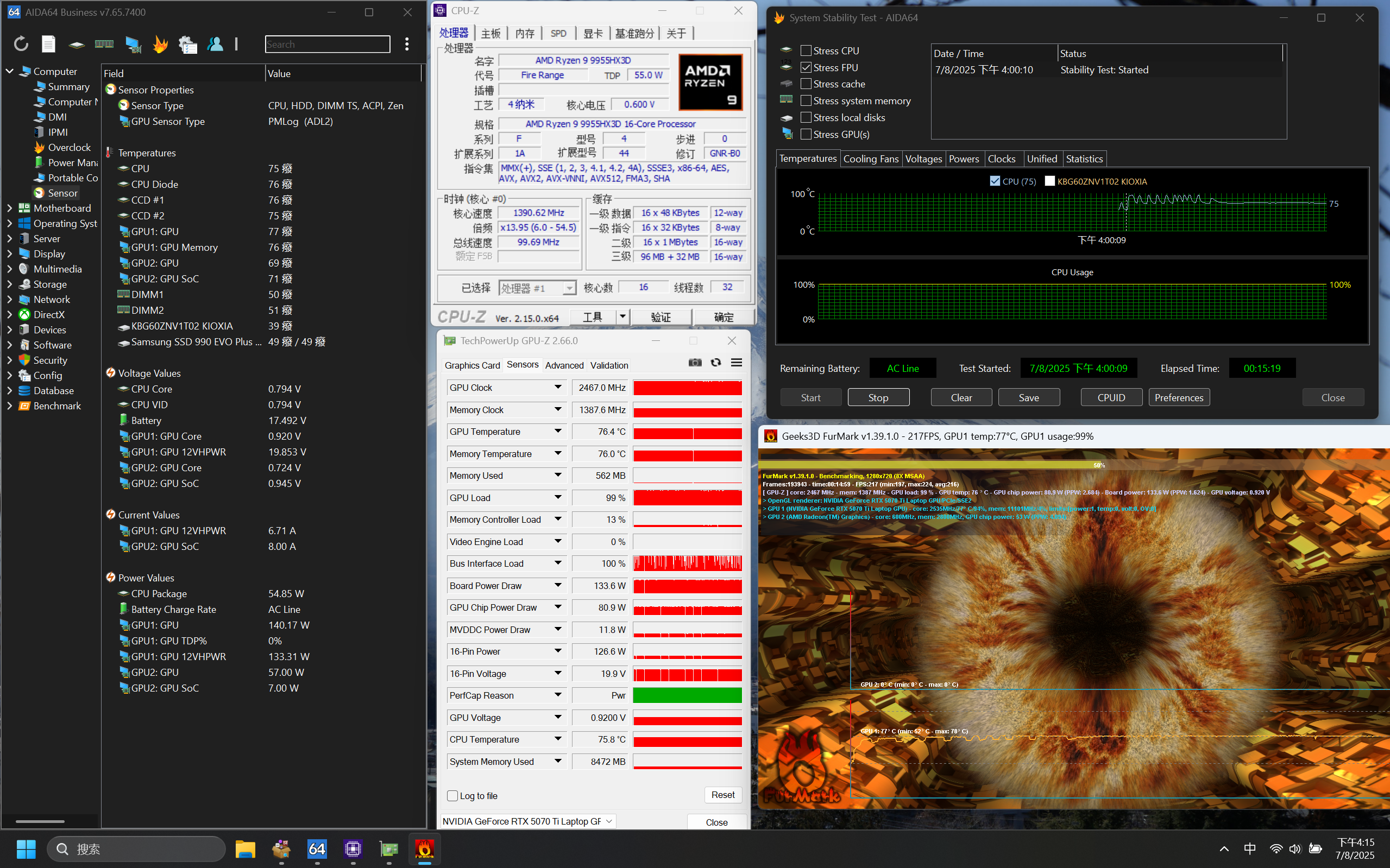
I bought a new computer and used it for about a week.
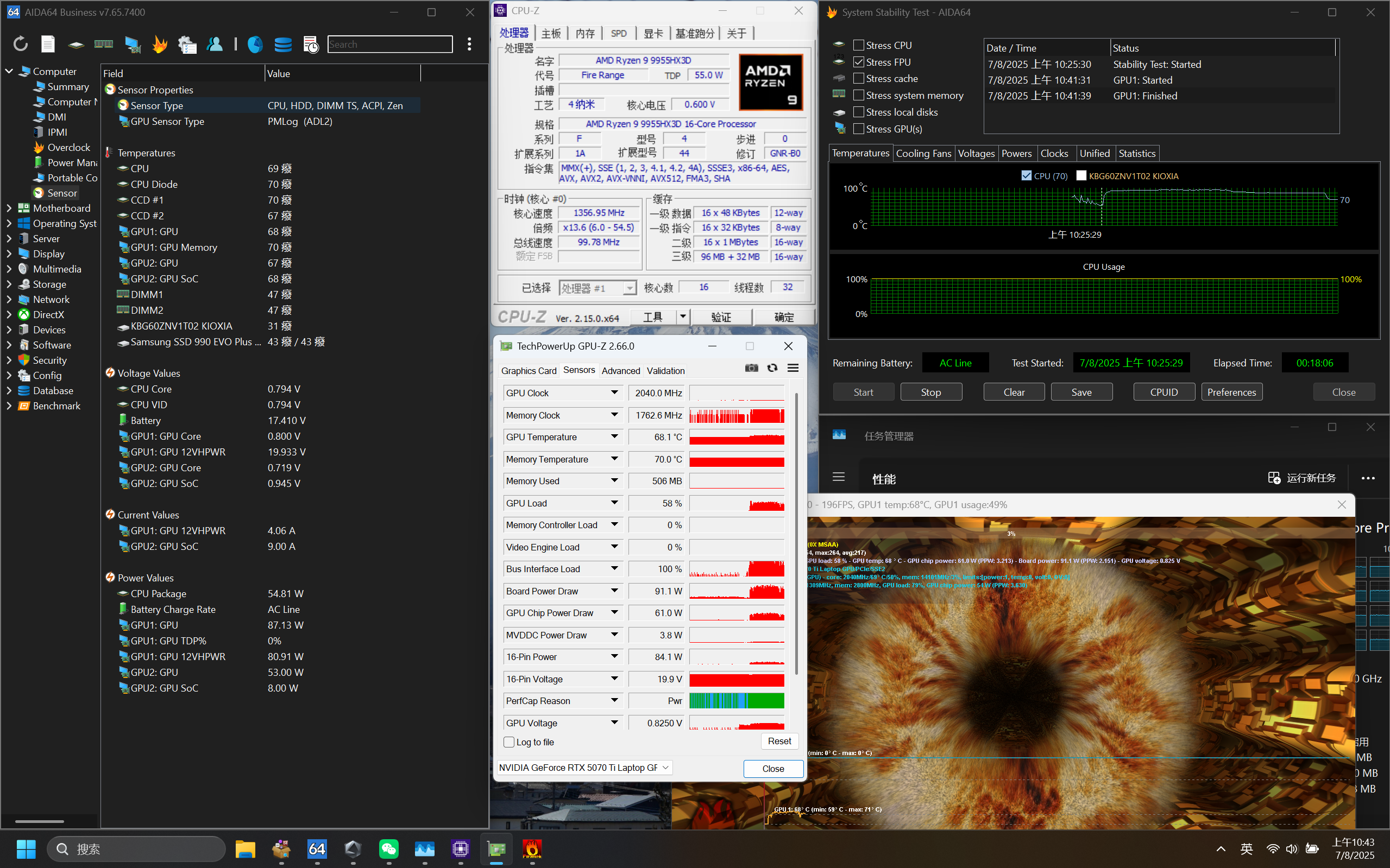
Before replacing the thermal paste, the CPU temperature consistently reached its power limit of 95°C at 125W. Under dual stress testing, the CPU released approximately 50W of power, reaching around 75°C, while the GPU, under X0 FurMark, consumed approximately 100W and reached around 68-70°C.
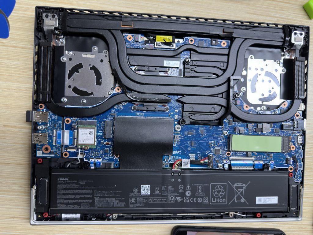
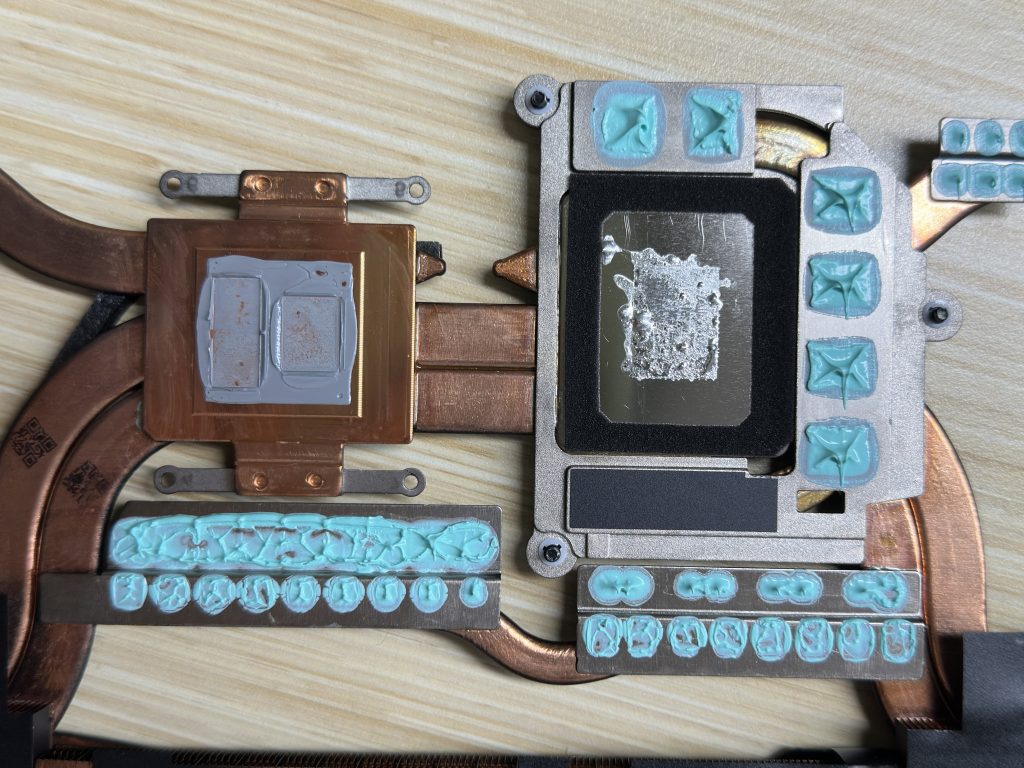
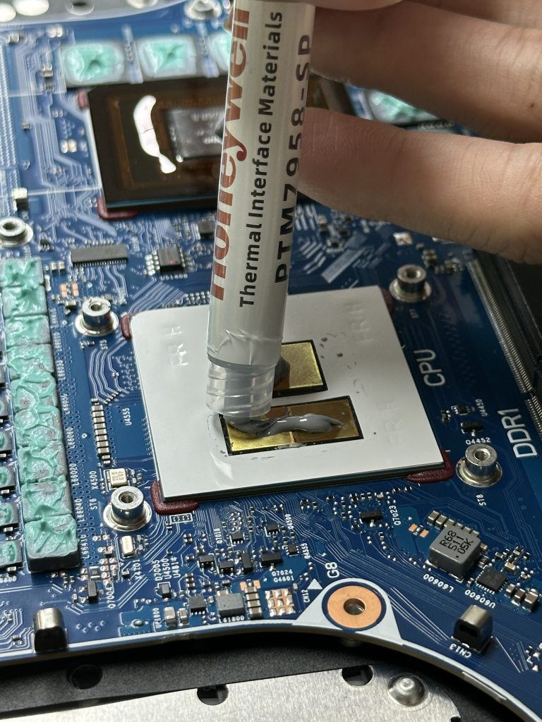
Begin replacing the Honeywell 7958SP. After removing all the screws, slightly twist the handles on both sides at the top; with a little force, the heatsink module can be removed. Be extra careful of any liquid metal residue remaining on the heatsink module.
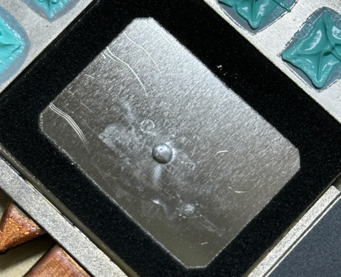
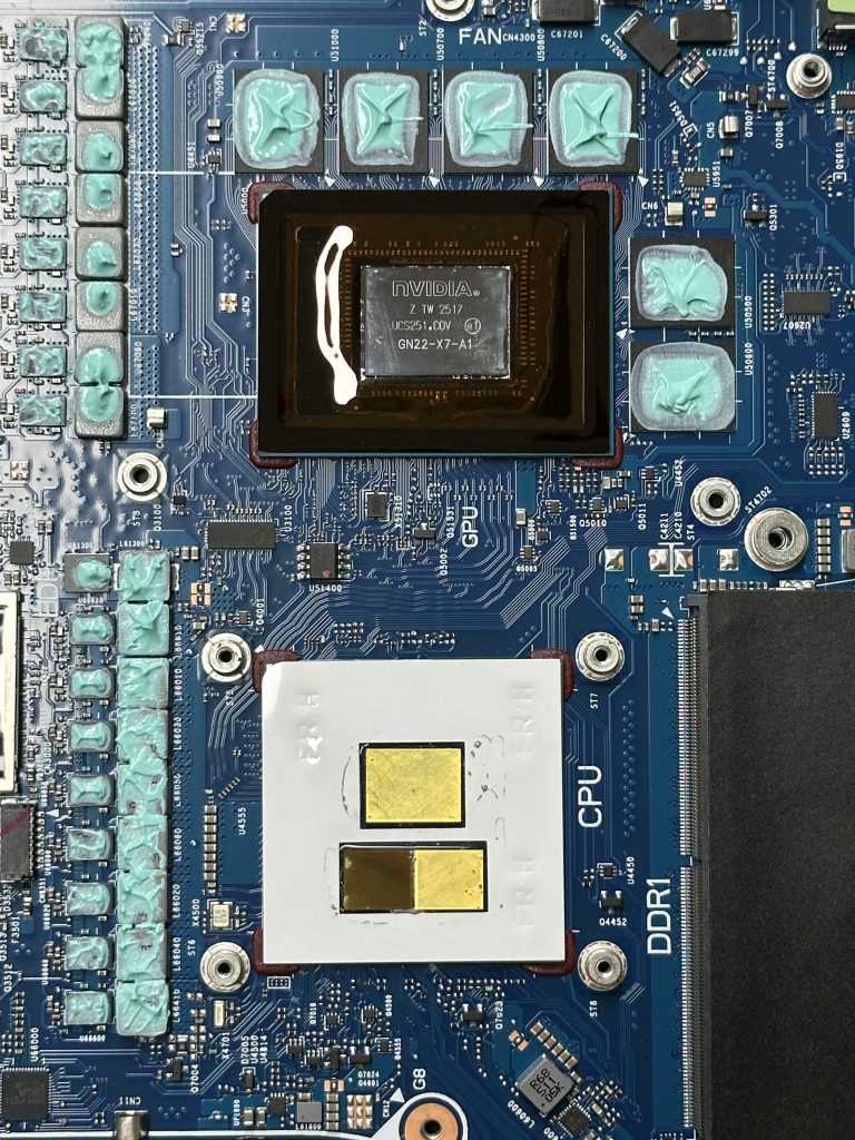
After disassembly, a significant amount of liquid metal was clearly observed to have leaked out, but this was likely due to movement during disassembly.
The heat dissipation module has foam pads to prevent liquid metal from overflowing, providing decent protection.
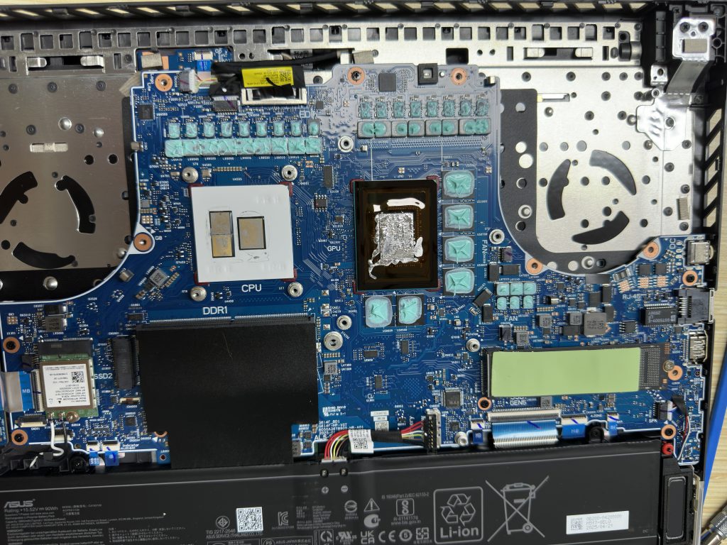
The liquid gold was removed using alcohol and cotton swabs. This process required patience and took about 20 minutes.
Finally, it was cleaned up.
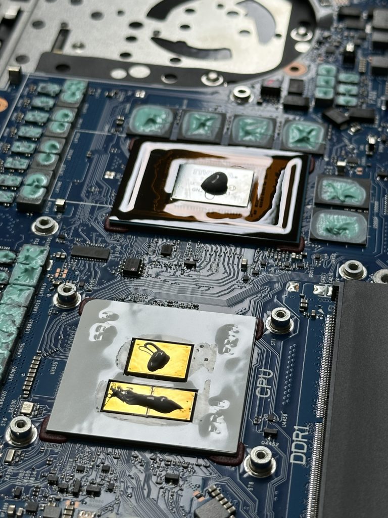
Then replace the thermal paste. Close the lid to finish.
Final roasting temperature compared to before replacementBasically the sameYes, you read that right, they are basically the same.
Furthermore, an additional nearly 4° elevation can be achieved by using a height adjustment pad. So why not?
FunctiongetCloudColor(viewVector, // Direction of gazeskyColor, // Background sky colorbasePos, // Ray originsamples, // Number of samplesumbral, // Threshold used to remove low noisebrightFactor, // High light intensitydither, // Jitter parametersCLOUD_PARAMS// Various cloud layer constants such as plane, center, and thickness):// 1. If your gaze is downward, return directly to the sky color.ifviewVector.y ≤ 0:returnskyColor// 2. Calculate the intersection points t0 and t1 of the ray with the upper and lower cloud planes.t0 = (CLOUD_BOTTOM - basePos.y) / viewVector.yt1 = (CLOUD_TOP - basePos.y) / viewVector.y// 3. Generate the sampling start point p and step size stepVp = basePos + viewVector * t0pEnd = basePos + viewVector * t1stepV = (pEnd - p) / samplesp += stepV * dither// Add a small amount of jitter to reduce banding// 4. Sample along the ray, accumulating "cloud thickness" cv and "first hit depth" dencv = 0// Cumulative cloud volume componentsden = 0// Relative position upon first entry into the cloud layer (0~1)firstHit = truetotalRange = (CLOUD_CENTER - CLOUD_BOTTOM) + (CLOUD_TOP - CLOUD_CENTER)foriin0 .. samples-1:// 4.1 Sampling noise (height field)noiseHi = sampleNoiseHeight(p.xz, timeOffsetHigh)noiseLo = sampleNoiseHeight(p.zx, timeOffsetLow) // Optional multi-layer mixingnoise = mixAndSmooth(noiseHi, noiseLo)// 4.2 Calculate the upper and lower boundaries of the cloud layer based on the thresholdv = (noise - umbral) / (1 - umbral)inf = CLOUD_CENTER - v * (CLOUD_CENTER - CLOUD_BOTTOM)sup = CLOUD_CENTER + v * (CLOUD_TOP - CLOUD_CENTER)// 4.3 Determine if the current sampling point py is inside the cloud layerifinf < p.y < sup:cv += min(stepLength, sup - inf)iffirstHit:den = (sup - p.y) / totalRangefirstHit = falseelseifwithinSoftEdge(p.y, inf, sup, CLOUD_EDGE_WIDTH):// Edge transition: Add a little accumulation softlycv += softBlendAmount(p.y, inf, sup) iffirstHit:den = (sup - p.y) / totalRangefirstHit = falsep += stepV// 5. Normalized cumulative value and depthopacity = clamp(cv / (2 * CLOUD_EDGE_WIDTH / viewVector.y), 0, 1)density = clamp(den, 0.0001, 1)// 6. Select colors by density: Low—Medium—Highifdensity < 0.33:baseColor = COL_SH// Cloud backgroundelseifdensity < 0.66:baseColor = COL_MD// Mid-layer colorelse:baseColor = COL_HI// Cloud Top Color// 7. Viewpoint Highlights: Only high-density areas are highlighted.ifdensity > 0.66:highlight = dot(computeNormal(density), -viewVector)baseColor = Mix(baseColor, COL_HI, highlight * brightFactor)// 8. Self-shadow: The thicker the shadow, the darker it is.baseColor *= Mix(1.0, 0.85, density^2 * 0.5)// 9. Edge Stroke: Enhance the contour based on the depth field gradientedgeFactor = computeEdgeFactor(opacity)baseColor = Mix(baseColor, OUTLINE_COLOR, edgeFactor * 0.3)// 10. Adjust the darkness at night according to the brightness of the sky.nightFactor = computeNightFactor(skyColor)baseColor *= nightFactor// 11. Final blend: Cloud-covered backgroundalpha = opacity * clamp((viewVector.y - 0.05) * 5.0, 0, 1)returnMix(skyColor, baseColor, alpha)
The notebook is divided into three parts: elementary, intermediate and advanced.
The beginner's chapter mainly introduces one-dimensional standard and non-standard FDTD theories.
The intermediate chapter will introduce the two-dimensional FDTD theory. The two-dimensional NS-FDTD theory improves the accuracy of solving Maxwell's equations by combining different finite difference models, which is one of the core of this method.
The advanced version will introduce the three-dimensional FDTD theory and apply it to conductive media (such as metals, plasmas, etc.) to study the propagation characteristics of electromagnetic waves in these materials.
Advantages of the NS-FDTD algorithm
Finite-difference time-domain (FDTD) is one of the most famous numerical algorithms for calculating electromagnetic wave propagation. The FDTD method can simulate structures of arbitrary shapes, nonlinear media, and can calculate the propagation of broadband electromagnetic waves. NS-FDTD reduces computing resources by optimizing the calculation of single-frequency waves, allowing higher-precision structures to be calculated with the same resource consumption. Using the NS-FDTD method, researchers have successfully and accurately simulated a special type of electromagnetic mode - Whispering Gallery Modes (WGM).
The whispering gallery mode refers to the phenomenon that electromagnetic waves or sound waves propagate near the inner wall of a circular, spherical or ring-shaped structure and circle around it many times without being easily scattered to the outside.
An intuitive example is that under the circular dome of St. Paul's Cathedral in London, if one person whispers softly on one side, another person on the other side, tens of meters away, can still hear it. This is because the sound waves propagate along the circular wall and stay on a specific path, thus reducing energy loss.
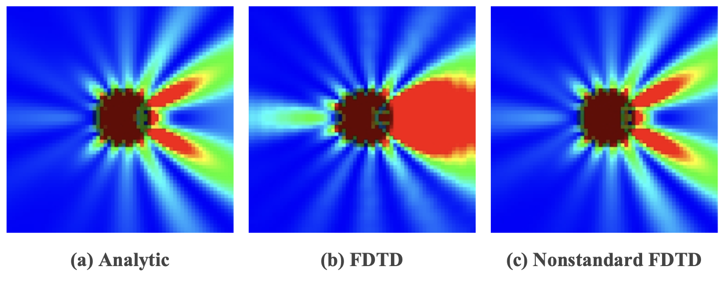
The traditional FDTD method often has large errors when calculating WGM, but the NS-FDTD method has higher accuracy, so the calculation results are closer to the theoretical values, as shown in the figure above.
(a) Figure: Analytical solution of Mie theory, used as a reference standard.
(b) Figure: Simulation results using the traditional FDTD method on a coarse grid deviate greatly from the theoretical values.
(c) Figure: Simulation using the NS-FDTD method on the same coarse grid. The results are highly consistent with the Mie theory and are significantly better than the traditional FDTD calculation results.
Beginner's Edition
First, we introduce the one-dimensional standard/non-standard FDTD theory. In computer simulation, additional considerations are required for numerical stability and boundary conditions.
1. Finite Difference Model
Many partial differential equations (PDEs) do not have analytical solutions, so they can only rely on numerical simulation. Finite difference method (FDM) is the most common numerical calculation method. The basic idea is to use differential expressions to approximate the solution of differential equations.
1.1 Forward Finite Difference (FFD)
To find the derivative of a one-dimensional function, first use Taylor Series Expansion to expand the function $f(x)$ at $x+\Delta x$: $$ f(x + \Delta x) = f(x) + \Delta x \frac{df(x)}{dx} + \frac{\Delta x^2}{2!} \frac{d^2 f(x)}{dx^2} + \cdots , \tag{1} $$ When $\Delta x$ is small enough, we can ignore the higher-order terms (i.e. $ \frac{\Delta x^2}{2!} \frac{d^2 f(x)}{dx^2} + \cdots $ ), and only keep the first-order derivative terms. Finally, we can get: $$ \frac{df(x)}{dx} \approx \frac{f(x+\Delta x) – f(x)}{\Delta x} . \tag{2} $$ Formula (2) is called the forward finite difference (FFD) approximation.
The term $\frac{\Delta x^2}{2!} \frac{d^2 f(x)}{dx^2} + \cdots$ is ignored in the Taylor expansion, so the truncation error is a first-order error, that is, $O(\Delta x) $ .
1.2 Backward Finite Difference (BFD)
Similarly, the expansion of the function $f(x)$ at $x – \Delta x$ is: $$ f(x – \Delta x) = f(x) – \Delta x \frac{df(x)}{dx} + \frac{\Delta x^2}{2!} \frac{d^2 f(x)}{dx^2} + \cdots . \tag{3} $$ Easy to get: $$ \frac{df(x)}{dx} \approx \frac{f(x) – f(x- \Delta x)}{\Delta x} . \tag{4} $$ The error is the same as above.
1.3 Central Finite Difference (CFD)
The previous two algorithms only use the current point and one adjacent point for calculation, so the accuracy is low. The center difference uses the two adjacent points before and after to improve the accuracy.
For the function $f(x)$, subtract formula (1) from formula (3), eliminate the second-order derivative term, and obtain: $$ f(x + \Delta x) – f(x – \Delta x) = 2\Delta x \frac{df}{dx} + O(\Delta x^3) . \tag{5} $$ Further sorting gives: $$ \frac{df}{dx} \approx \frac{f(x + \Delta x) – f(x – \Delta x)}{2\Delta x} . \tag{6} $$ Some textbooks use $ \Delta x/2 $ to replace $ \Delta x $ to obtain formula (7). The two are actually equivalent. $$ \frac{df}{dx} \approx \frac{f(x + \Delta x/2) – f(x – \Delta x/2)}{\Delta x} . \tag{7} $$ Both of the above formulas are called second-orderCentral finite differenceformula.
In addition, for the function $f(x)$, adding formula (1) to formula (3) and eliminating the first-order derivative term, we can obtain: $$ f(x+ \Delta) + f(x- \Delta) = 2f(x) + \Delta x^2 \frac{d^2 f}{dx^2} + O(\Delta x^4). \tag{8} $$ After sorting, we get: $$ \frac{d^2 f}{dx^2} \approx \frac{f(x + \Delta x) – 2f(x) + f(x – \Delta x)}{\Delta x^2} \tag{9} $$
1.4 Higher-Order Finite Difference
In the finite difference method, the calculation accuracy is improved by increasing the number of sampling points to obtain a higher-order difference formula.
In order to improve the accuracy, two additional sampling points $x + 2\Delta x, x – 2\Delta x$ are added on the basis of the second-order central finite difference method, and Taylor expansion is performed here:
For the right-hand side points, the Taylor expansion is: $$ f(x+2\Delta x) = f(x) + 2\Delta x\frac{df(x)}{dx} + 2\Delta x^2 \frac{d^2f(x)}{dx^2}+O(\Delta x^3) , \tag{10} $$ Similarly, $$ f(x – 2\Delta x) = f(x) – 2\Delta x \frac{df(x)}{dx} + 2\Delta x^2 \frac{d^2 f(x)}{dx^2} + O(\Delta x^3) . \tag{11} $$ By linear combination (for example, inverting formula (11) and halving it, and adding the two formulas together), we can eliminate the high-order error terms and obtain: $$ \frac{d^2 f(x)}{dx^2} \approx \frac{1}{\Delta x^2} \left[ \frac{4}{3} (f(x + \Delta x) + f(x – \Delta x)) – \frac{1}{12} (f(x + 2\Delta x) + f(x – 2\Delta x)) – \frac{5}{2} f(x) + \cdots \right] . \tag{12} $$ This model uses four points and reduces the error by weighted averaging, but it brings potential problems such as numerical instability.
When we replace differential equations with higher-order finite differences, we introduce additional numerical solutions, called spurious solutions, which do not actually exist but are caused by the discretization properties of higher-order difference equations.
For example, a first-order differential equation such as $ \frac{df}{dx} = f(x) $ usually has one independent solution, a second-order differential equation such as the wave equation $\frac{d^2f}{dx^2}=k^2f(x)$ usually has two independent solutions (two free parameters), a fourth-order differential equation will have four independent solutions, and so on.
In numerical calculations, if a fourth-order finite difference method is used to approximate a second-order differential equation, the end of the difference equation will be forcibly raised, resulting in additional spurious solutions. These additional solutions do not correspond to the original physical system.
In particular, the second-order differential wave equation describing electromagnetic wave propagation should be solved using the second-order central finite difference method rather than higher-order methods.
2. One-dimensional wave equation
To simulate the propagation of waves on a computer, numerical methods are needed for approximate calculations, among which the finite difference time domain method plays a powerful role.
The mathematical expression of the one-dimensional wave equation is: $$ \frac{\partial^2 \psi}{\partial t^2} = v^2 \frac{\partial^2 \psi}{\partial x^2} , \tag{1} $$ Where $\psi(x,t)$ represents the amplitude of the wave, $v$ is the speed of wave propagation (light in a vacuum is $3 \times 10^8$ m/s).
The physical meaning of this equation is that the change of waves is related to the change of time and space.
For an infinitely long wave medium, the solution is usually a traveling wave of a very simple form: $$ \psi(x,t) = A \cos(kx – \omega t) + B \sin(kx – \omega t) . \tag{2} $$ This situation applies to electromagnetic waves propagating in free space. For example, if the boundary is fixed, the traveling wave can be expanded by a sine function: $$ \psi(x,t) = \sum_{n} A_n \sin(k_n x) \cos(\omega_n t). \tag{3} $$ However, if the boundary is irregular, such as electromagnetic waves reflecting on the ground, water waves hitting the coastline, sound waves propagating in multiple rooms, etc., it cannot be simply expanded into a sine or exponential form, and the analytical solution will be extremely complicated. For example, sound waves will have different reflection paths when they contact walls of different media, making it impossible to directly solve the propagation path of the sound waves.
Analytical solutions usually assume that the wave speed $v$ is constant, that is, the wave propagates in a homogeneous medium. But in reality, waves travel through inhomogeneous media, such as sound waves that have different propagation speeds in rooms of different temperatures. In these cases, the wave equation becomes a variable coefficient partial differential equation, such as: $$ \frac{\partial^2 \psi}{\partial t^2} = v(x)^2 \frac{\partial^2 \psi}{\partial x^2} , \tag{4} $$ The speed $v$ will change with the position $x$, which makes it impossible to directly use Fourier transform to obtain the analytical value.
Or there is an excitation source on the right side of the wave equation, that is, multiple waveforms may have different sources interfering with each other. In this case, it is also difficult to find an analytical solution.
And in the real world, the propagation of energy will cause losses, so it is necessary to introduce loss terms into the wave equation. At this time, the wave equation will become a nonlinear equation or a high-order differential equation, making it impossible to solve directly.
Therefore, we introduce the finite difference time domain method to solve these problems.
2.1 Standard FDTD algorithm
Since computers cannot directly calculate continuous mathematical equations, they needDiscretization, which divides space and time into grids, and then lets the computer gradually calculate the fluctuations of each grid.
In continuous form, the one-dimensional wave equation $$ \frac{\partial^2 \psi}{\partial t^2} = v^2 \frac{\partial^2 \psi}{\partial x^2} , \tag{1*} $$ The equivalent form is $$ \left( \frac{\partial^2}{\partial t^2} – v^2 \frac{\partial^2}{\partial x^2} \right) \psi(x,t) = 0. \tag{5} $$ Therefore, using the interval $\Delta x$ to discretize space, each point is represented by the index $i$$x = i\Delta x$; using the interval $\Delta t$ to discretize time, each moment is represented by the miniature $n$$t = n\Delta t$, where $n$ are all integers. So the wave function is written as: $$ \psi_i^n = \psi(i\Delta x, n\Delta t) . \tag{6} $$ The derivative of the wave function is then calculated using the central finite difference method.
The central finite difference approximation of the second-order partial derivative functions in time and space directions is $$ \frac{\partial^2 \psi}{\partial t^2} \approx \frac{\psi_i^{n+1} – 2\psi_i^n + \psi_i^{n-1}}{\Delta t^2} , \tag{7} $$
where $\psi_{i+1}^{n}$ is the fluctuation value of the adjacent grid point on the right.
Substituting formula (7) and formula (8) into the wave equation (formula (1)), we obtain formula (9). $$ \frac{\psi_i^{n+1} – 2\psi_i^n + \psi_i^{n-1}}{\Delta t^2} = v^2 \frac{\psi_{i+1}^{n} – 2\psi_i^n + \psi_{i-1}^{n}}{\Delta x^2} , \tag{9} $$ After sorting out, we get the standard 1D FDTD calculation formula.1D standard finite difference time domain (FDTD) algorithm: $$ \psi_i^{n+1} = 2\psi_i^n – \psi_i^{n-1} + \left( \frac{v^2 \Delta t^2}{\Delta x^2} \right) (\psi_{i+1}^{n} – 2\psi_i^n + \psi_{i-1}^{n}) . \tag{10} $$ This formula depends on the calculation of the two step points before and after in time and space. In other words, the state of the current point is affected by the adjacent points.
2.2 Non-standard FDTD algorithm
In the standard FDTD method, the wave equation is discretized using central differences. However, this method hasNumerical dispersionProblem: There will be large errors when the grid is coarse.
The non-standard FDTD algorithm solves the above problems. NS-FDTD makes special treatment for monochromatic waves, ensuring accuracy even if the values are discrete.
First, suppose that we are studying a certain monochromatic wave $$ \psi(x,t) \;=\; e^{\,i(kx – \omega t)}, \tag{11} $$ where $k$ is the wave number ($k = 2\pi / \lambda$) and $\omega$ is the angular frequency ($\omega = 2\pi f$).
The spatial differential of formula (11) in the continuous case is $$ \frac{\partial \psi}{\partial x} \;=\; i\,k\, \psi(x,t). \tag{12} $$ For example, if we use standard differences directly to calculate $\Delta_x \psi(x,t)$, we get $$ \Delta_x \psi(x,t) = \psi(x+\Delta x,t) – \psi(x,t) = e^{\,i(kx – \omega t)}\bigl(e^{\,i\,k\,\Delta x} – 1\bigr) , \tag{13} $$ It is not consistent with the real differential. It can only be approximated when $\Delta x$ is small enough. In other words, if the grid is coarse, the so-called error will occur.
NS-FDTD introduces the correction factor $s(\Delta x)$ to minimize the error of the discrete operator $$ \Delta_x \psi(x,t) \approx s(\Delta x)\,\frac{\partial \psi(x,t)}{\partial x}. \tag{14} $$ This $s(\Delta x)$ is determined by the phase change at $\Delta x$. For example, our goal is $$ \Delta_x \psi(x,t) = \psi(x+\Delta x,t) – \psi(x,t) . \tag{15} $$ Then the error factor is derived from formulas (12), (13), (14), and (15): $$ s(\Delta x)
=\frac{\Delta_x \psi(x,t)}{\partial_x \psi(x,t)}
\frac{e^{\,i\,k\,\Delta x} – 1}{i\,k\,\Delta x}
\times \Delta x
\frac{e^{ik\Delta x} – 1}{ik}. \tag{16} $$ By using Euler's formula, the error factor is simplified to $$ s(\Delta x) = \frac{2}{k}\,\sin!\Bigl(\frac{k\,\Delta x}{2}\Bigr)\,e^{\,i\,\frac{k\,\Delta x}{2}} . \tag{17} $$ Note that when $\Delta x \to 0$, the nonstandard difference degenerates back to the case of "standard central difference", which is almost consistent with the true derivative approximation. In fact, formula (17) contains two parts: phase factor and amplitude, the former corresponds to the exponential part.
Similarly, the correction function in the time direction is derived $$ s(\Delta t) = \frac{2}{\omega}\,\sin\Bigl(\frac{\omega\,\Delta t}{2}\Bigr)e^{-\,i\omega\,\Delta t/2}. \tag{18} $$ To summarize, we start with the wave equation, discretize space and time, approximate it with the central difference, and then introduce the correction function (the exponential term of the correction function is actually handled implicitly) $$ \frac{\psi_i^{n+1} – 2\psi_i^n + \psi_i^{n-1}}{\left(\frac{2}{\omega} \sin(\omega \Delta t / 2)\right)^2} = v^2 \frac{\psi_{i+1}^{n} – 2\psi_i^n + \psi_{i-1}^{n}}{\left(\frac{2}{k} \sin(k \Delta x / 2)\right)^2}. \tag{19} $$ After sorting, we get $$ \psi_i^{n+1} = -\psi_i^{n-1} + \left(2 + u_{\text{NS}}^2 d_x^2 \right) \psi_i^n , \tag{20} $$ in $$ u_{\text{NS}} = \frac{\sin(\omega \Delta t / 2)}{\sin(k \Delta x / 2)} . \tag{21} $$
3. One-dimensional FDTD stability
When doing numerical simulation, we hope that the time step $\Delta t$ is as large as possible to reduce the total number of calculation steps, but it cannot exceed a certain limit, otherwise the numerical solution will diverge. How is this limit derived?